
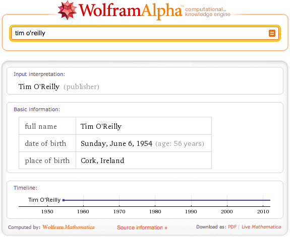
Throughout this chapter, it’s been implied that analytic approaches that exhibit a deeper understanding of the data can be dramatically more powerful than approaches that simply treat each token as an opaque symbol. But what does “a deeper understanding” of the data really mean? One interpretation is being able to detect the entities in documents and using those entities as the basis of analysis, as opposed to document-centric analysis involving keyword searches or interpreting a search input as a particular type of entity and customizing results accordingly. Although you may not have thought about it in those terms, this is precisely what emerging technologies such as WolframAlpha do at the presentation layer. For example, a search for “tim o’reilly” in WolframAlpha returns results that imply an understanding that the entity being searched for is a person; you don’t just get back a list of documents containing the keywords (see Figure 8-3). Regardless of the internal technique that’s used to accomplish this end, the resulting user experience is dramatically more powerful because the results conform to a format that more closely satisfies the user’s expectations.
Although it’s beyond the scope of this chapter to ponder the various possibilities of entity-centric analysis, it’s well within our scope and quite appropriate to present a means of extracting the entities from a document, which can then be used for various analytic purposes. Assuming the sample flow of an NLP pipeline as presented earlier in this chapter, one approach you could take would be to simply extract all the nouns and noun phrases from the document and index them as entities appearing in the documents—the important underlying assumption being that nouns and noun phrases (or some carefully constructed subset thereof) qualify as entities of interest. This is actually a very fair assumption to make and a good starting point for entity-centric analysis, as the following sample listing demonstrates. Note that for results annotated according to Penn Treebank conventions, any tag beginning with ‘NN’ is some form of a noun or noun phrase. A full listing of the Penn Treebank Tags is available online.
Example 8-5 analyzes the part-of-speech tags that are applied to tokens, and identifies nouns and noun phrases as entities. In data-mining parlance, finding the entities in a text is called entity extraction.
Example 8-5. Extracting entities from a text with NLTK (blogs_and_nlp__extract_entities.py)
# -*- coding: utf-8 -*-

import sys
import nltk
import json

# Load in output from blogs_and_nlp__get_feed.py

BLOG_DATA = sys.argv[1]
blog_data = json.loads(open(BLOG_DATA).read())

for post in blog_data:

    sentences = nltk.tokenize.sent_tokenize(post['content'])
    tokens = [nltk.tokenize.word_tokenize(s) for s in sentences]
    pos_tagged_tokens = [nltk.pos_tag(t) for t in tokens]

    # Flatten the list since we're not using sentence structure
    # and sentences are guaranteed to be separated by a special
    # POS tuple such as ('.', '.')

    pos_tagged_tokens = [token for sent in pos_tagged_tokens for token in sent]

    all_entity_chunks = []
    previous_pos = None
    current_entity_chunk = []
    for (token, pos) in pos_tagged_tokens:

        if pos == previous_pos and pos.startswith('NN'):
            current_entity_chunk.append(token)
        elif pos.startswith('NN'):
            if current_entity_chunk != []:

                # Note that current_entity_chunk could be a duplicate when appended,
                # so frequency analysis again becomes a consideration

                all_entity_chunks.append((' '.join(current_entity_chunk), pos))
            current_entity_chunk = [token]

        previous_pos = pos

    # Store the chunks as an index for the document
    # and account for frequency while we're at it...

    post['entities'] = {}
    for c in all_entity_chunks:
        post['entities'][c] = post['entities'].get(c, 0) + 1

    # For example, we could display just the title-cased entities

    print post['title']
    print '-' * len(post['title'])
    proper_nouns = []
    for (entity, pos) in post['entities']:
        if entity.istitle():
            print '	%s (%s)' % (entity, post['entities'][(entity, pos)])
    print
Note
You may recall from the description of “extraction” in A Typical NLP Pipeline with NLTK that NLTK provides an
nltk.batch_ne_chunk function that
attempts to extract named entities from POS-tagged tokens. You’re
welcome to use this capability directly, but you may find that your
mileage varies with the out-of-the-box models that back the
implementation. A discussion of improving the implementation that
ships with NLTK is outside the scope of this chapter.
Sample output for the listing is presented in Example 8-6. It provides results that are quite meaningful and would make great suggestions for tags by an intelligent blogging platform. For a larger corpus than we’re working with in this example, a tag cloud would also be an obvious candidate for visualizing the data. (Recall that Visualizing Tweets with Tricked-Out Tag Clouds introduced an easy-to-use but very powerful tag cloud that you could easily adapt to work here.)
Example 8-6. Sample results from Example 8-5
The Louvre of the Industrial Age
--------------------------------
	Paris (1)
	Henry Ford Museum (1)
	Vatican Museum (1)
	Museum (1)
	Thomas Edison (2)
	Hermitage (1)
	Uffizi Gallery (1)
	Ford (2)
	Santa Rosa (1)
	Dearborn (1)
	Makerfaire (1)
	Berlin (1)
	Marc (2)
	Makerfaire (1)
	Rome (1)
	Henry Ford (1)
	Ca (1)
	Louvre (1)
	Detroit (2)
	St. Petersburg (1)
	Florence (1)
	Marc Greuther (1)
	Makerfaire Detroit (1)
	Luther Burbank (2)
	Make (1)
	Dale Dougherty (1)
    Louvre (1)
Could we have discovered the same list of terms by more blindly analyzing the lexical characteristics (such as use of capitalization) of the sentence? Perhaps, but keep in mind that this technique can also capture nouns and noun phrases that are not indicated by title case. Case is indeed an important feature of the text that can generally be exploited to great benefit, but there are other interesting entities in the sample text that are all lowercase (for example, “chief curator”, “locomotives”, and “lightbulbs”).
Although the list of entities certainly doesn’t convey the overall meaning of the text as effectively as the summary we computed earlier, identifying these entities can be extremely valuable for analysis since they have meaning at a semantic level and are not just frequently occurring words. In fact, the frequencies of most of the terms displayed in the sample output are quite low. Nevertheless, they’re important because they have a grounded meaning in the text—namely, they’re people, places, things, or ideas, which are generally the substantive information in the data.
It’s not much of a leap at this point to think that it would be another major step forward to take into account the verbs and compute triples of the form subject-verb-object so that you know which entities are interacting with which other entities, and the nature of those interactions. Such triples would lend themselves to visualizing object graphs of documents, which could potentially be skimmed much faster than reading the documents themselves. Better yet, imagine taking multiple object graphs derived from a set of documents and merging them to get the gist of the larger corpus. This exact technique is very much an area of active research and has tremendous applicability for virtually any situation suffering from the information-overload problem. But as will be illustrated, it’s an excruciating problem for the general case and not for the faint of heart.
Assuming a part-of-speech tagger has identified the following parts
of speech from a sentence and emitted output such as [('Mr.', 'NNP'), ('Green', 'NNP'), ('killed', 'VBD'),
('Colonel', 'NNP'), ('Mustard', 'NNP'), ...], an index storing
subject-predicate-object tuples of the form ('Mr.
Green', 'killed', 'Colonel Mustard') would be easy to compute.
However, the reality of the situation is that you’re very unlikely to run
across actual POS-tagged data with that level of simplicity—unless you’re
planning to mine children’s books (something that’s not actually a bad
idea for beginners). For example, consider the tagging emitted from NLTK
for the first sentence from the blog post printed earlier in this chapter
as an arbitrary and realistic piece of data you might like to translate
into an object graph:
This morning I had the chance to get a tour of The Henry Ford Museum in Dearborn, MI, along with Dale Dougherty, creator of Make: and Makerfaire, and Marc Greuther, the chief curator of the museum.
The simplest possible triple that you might expect to distill from
that sentence is ('I', 'get', 'tour'),
but even if you got that back, it wouldn’t convey that Dale Dougherty also
got the tour, or that Mark Greuther was involved. The POS-tagged data
should make it pretty clear that it’s not quite so straightforward to
arrive at any of those interpretations, either, because the sentence has a
very rich structure:
[(u'This', 'DT'), (u'morning', 'NN'), (u'I', 'PRP'), (u'had', 'VBD'), (u'the', 'DT'),(u'chance', 'NN'), (u'to', 'TO'), (u'get', 'VB'), (u'a', 'DT'), (u'tour', 'NN'),(u'of', 'IN'), (u'The', 'DT'), (u'Henry', 'NNP'), (u'Ford', 'NNP'), (u'Museum', 'NNP'),(u'in', 'IN'), (u'Dearborn', 'NNP'), (u',', ','), (u'MI', 'NNP'), (u',', ','),(u'along', 'IN'), (u'with', 'IN'), (u'Dale', 'NNP'), (u'Dougherty', 'NNP'), (u',',','), (u'creator', 'NN'), (u'of', 'IN'), (u'Make', 'NNP'), (u':', ':'), (u'and', 'CC'),(u'Makerfaire', 'NNP'), (u',', ','), (u'and', 'CC'), (u'Marc', 'NNP'), (u'Greuther','NNP'), (u',', ','), (u'the', 'DT'), (u'chief', 'NN'), (u'curator', 'NN'), (u'of','IN'), (u'the', 'DT'), (u'museum', 'NN'), (u'.', '.')]
It’s doubtful whether even a state-of-the-art solution would be capable of emitting meaningful triples in this case, given the complex nature of the predicate “had a chance to get a tour”, and that the other actors involved in the tour are listed in a phrase appended to the end of the sentence. Strategies for constructing these triples are well outside the scope of this book, but in theory, you should be able to use reasonably accurate POS tagging information to take a good stab at it. The difficulty of this task was pointed out not to discourage you, but to provide a realistic view of the complexity of NLP in general so that you know what you’re getting into when you decide to tackle the problem of computing triples for the general case. It can be a lot of work, but the results are well worth it.
All that said, the good news is that you can actually do a lot of interesting things by distilling just the entities from text and using them as the basis of analysis, as demonstrated earlier. You can very easily produce triples from text on a per-sentence basis, where the “predicate” of each triple is a notion of a generic relationship signifying that the subject and object “interacted” with one another. Example 8-7 is a refactoring of Example 8-5 that collects entities on a per-sentence basis, which could be quite useful for computing the interactions between entities using a sentence as a context window.
Example 8-7. Discovering interactions between entities (blogs_and_nlp__extract_interactions.py)
# -*- coding: utf-8 -*-

import sys
import nltk
import json

def extract_interactions(txt):
    sentences = nltk.tokenize.sent_tokenize(txt)
    tokens = [nltk.tokenize.word_tokenize(s) for s in sentences]
    pos_tagged_tokens = [nltk.pos_tag(t) for t in tokens]

    entity_interactions = []
    for sentence in pos_tagged_tokens:

        all_entity_chunks = []
        previous_pos = None
        current_entity_chunk = []

        for (token, pos) in sentence:

            if pos == previous_pos and pos.startswith('NN'):
                current_entity_chunk.append(token)
            elif pos.startswith('NN'):
                if current_entity_chunk != []:
                    all_entity_chunks.append((' '.join(current_entity_chunk),
                            pos))
                current_entity_chunk = [token]

            previous_pos = pos

        if len(all_entity_chunks) > 1:
            entity_interactions.append(all_entity_chunks)
        else:
            entity_interactions.append([])

    assert len(entity_interactions) == len(sentences)

    return dict(entity_interactions=entity_interactions,
                sentences=sentences)

if __name__ == '__main__':

    # Read in output from blogs_and_nlp__get_feed.py

    BLOG_DATA = sys.argv[1]
    blog_data = json.loads(open(BLOG_DATA).read())

    # Display selected interactions on a per-sentence basis

    for post in blog_data:

        post.update(extract_interactions(post['content']))

        print post['title']
        print '-' * len(post['title'])
        for interactions in post['entity_interactions']:
            print '; '.join([i[0] for i in interactions])
        print
The results from this listing, presented in Example 8-8, highlight something very important about the nature of unstructured data analysis: it’s messy!
Example 8-8. Sample output from Example 8-7
The Louvre of the Industrial Age
--------------------------------
morning; chance; tour; Henry Ford Museum; Dearborn; MI; Dale Dougherty; creator;
Make; Makerfaire; Marc Greuther; chief curator

tweet; Louvre

"; Marc; artifact; museum; block; contains; Luther Burbank; shovel; Thomas Edison…

Luther Burbank; course; inventor; treasures; nectarine; Santa Rosa

Ford; farm boy; industrialist; Thomas Edison; friend

museum; Ford; homage; transformation; world

machines; steam; engines; coal; generators; houses; lathes; precision; lathes;
makerbot; century; ribbon glass machine; incandescent; lightbulbs; world; combine;
harvesters; railroad; locomotives; cars; airplanes; gas; stations; McDonalds;
restaurant; epiphenomena

Marc; eye; transformation; machines; objects; things

advances; engineering; materials; workmanship; design; years

years; visit; Detroit; museum; visit; Paris; Louvre; Rome; Vatican Museum; Florence;
Uffizi Gallery; St. Petersburg; Hermitage; Berlin

world; museums

Museum; Makerfaire Detroit

reach; Detroit; weekend

day; Makerfaire; day
A certain amount of noise in the results is almost inevitable, but realizing results that are highly intelligible and useful—even if they do contain a manageable amount of noise—is a very worthy aim. The amount of effort required to achieve pristine results that are nearly noise-free can be immense. In fact, in most situations, this is downright impossible because of the inherent complexity involved in natural language and the limitations of most currently available toolkits, such as NLTK. If you are able to make certain assumptions about the domain of the data or have expert knowledge of the nature of the noise, you may be able to devise heuristics that are effective without risking an unacceptable amount of potential information loss. But it’s a fairly difficult proposition.
Still, the interactions do provide a certain amount of “gist” that’s valuable. For example, how closely would your interpretation of “morning; chance; tour; Henry Ford Museum; Dearborn; MI; Dale Dougherty; creator; Make; Makerfaire; Marc Greuther; chief curator” align with the meaning in the original sentence?
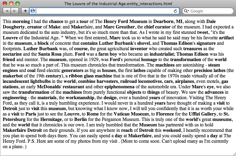
As was the case with our previous adventure in summarization, displaying markup that can be visually skimmed for inspection is also quite handy. A simple modification to the script’s output is all that’s necessary to produce the result shown in Figure 8-4 (see Example 8-9).
Example 8-9. Modification of script from Example 8-7 (blogs_and_nlp__extract_interactions_markedup_output.py)
# -*- coding: utf-8 -*-

import os
import sys
import nltk
import json
from blogs_and_nlp__extract_interactions import extract_interactions

HTML_TEMPLATE = """<html>
    <head>
        <title>%s</title>
        <meta http-equiv="Content-Type" content="text/html; charset=UTF-8"/>
    </head>
    <body>%s</body>
</html>"""

if __name__ == '__main__':

    # Read in output from blogs_and_nlp__get_feed.py

    BLOG_DATA = sys.argv[1]
    blog_data = json.loads(open(BLOG_DATA).read())

    # Marked up version can be written out to disk

    if not os.path.isdir('out/interactions'):
        os.makedirs('out/interactions')

    for post in blog_data:

        post.update(extract_interactions(post['content']))

        # Display output as markup with entities presented in bold text

        post['markup'] = []

        for sentence_idx in range(len(post['sentences'])):

            s = post['sentences'][sentence_idx]
            for (term, _) in post['entity_interactions'][sentence_idx]:
                s = s.replace(term, '<strong>%s</strong>' % (term, ))

            post['markup'] += [s]

        filename = post['title'] + '.entity_interactions.html'
        f = open(os.path.join('out', 'interactions', filename), 'w')
        html = HTML_TEMPLATE % (post['title'] + ' Interactions', ' '.join(post['markup']),)
        f.write(html.encode('utf-8'))
        f.close()

        print >> sys.stderr, "Data written to", f.name
As a consideration for the “interested reader,” it would be worthwhile to perform additional analyses to identify the sets of interactions for a larger body of text and to find co-occurrences in the interactions. You could also very easily adapt some of the Graphviz or Protovis output from Chapter 1 to visualize a graph of the interactions where edges don't necessary have any labels. The example file http://github.com/ptwobrussell/Mining-the-Social-Web/blob/master/python_code/introduction__retweet_visualization.py would make a very good starting point.
Even without knowing the specific nature of the interaction, there’s still a lot of value in just knowing the subject and the object. And if you’re feeling ambitious and are comfortable with a certain degree of messiness and lack of precision, by all means you can attempt to fill in the missing verbs!
When you’ve done a lot of data mining, you’ll eventually want to start quantifying the quality of your analytics. This is especially the case with text mining. For example, if you began customizing the basic algorithm for extracting the entities from unstructured text, how would you know whether your algorithm was getting more or less performant with respect to the quality of the results? While you could manually inspect the results for a small corpus and tune the algorithm until you were satisfied with them, you’d still have a devil of a time determining whether your analytics would perform well on a much larger corpus or a different class of document altogether—hence, the need for a more automated process.
An obvious starting point is to randomly sample some documents and create a “golden set” of entities that you believe are absolutely crucial for a good algorithm to extract from them and use this list as the basis of evaluation. Depending on how rigorous you’d like to be, you might even be able to compute the sample error and use a statistical device called a confidence interval[55] to predict the true error with a sufficient degree of confidence for your needs.
However, what exactly is the calculation you should be computing based on the results of your extractor and golden set in order to compute accuracy? A very common calculation for measuring accuracy is called the F1 score, which is defined in terms of two concepts called precision and recall[56] as:
where:
and:
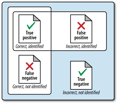
In the current context, precision is a measure of exactness that reflects “false positives,” and recall is a measure of completeness that reflects “true positives.” The following list clarifies the meaning of these terms in relation to the current discussion in case they’re unfamiliar or confusing:
Given that precision is a measure of exactness that quantifies false positives, it is defined as precision = TP / (TP + FP). Intuitively, if the number of false positives is zero, the exactness of the algorithm is perfect and the precision yields a value of 1.0. Conversely, if the number of false positives is high and begins to approach or surpass the value of true positives, precision is poor and the ratio approaches zero. As a measure of completeness, recall is defined as TP / (TP + FN) and yields a value of 1.0, indicating perfect recall, if the number of false negatives is zero. As the number of false negatives increases, recall approaches zero. Note that by definition, F1 yields a value of 1.0 when precision and recall are both perfect, and approaches zero when both precision and recall are poor. Of course, what you’ll find out in the wild is that it’s generally a trade-off as to whether you want to boost precision or recall, because it’s very difficult to have both. If you think about it, this makes sense because of the trade-offs involved with false positives and false negatives (see Figure 8-5).
To put all of this into perspective, let’s consider the classic (by now anyway) sentence, “Mr. Green killed Colonel Mustard in the study with the candlestick” and assume that an expert has determined that the key entities in the sentence are “Mr. Green”, “Colonel Mustard”, “study”, and “candlestick”. Assuming your algorithm identified these four terms and only these four terms, you’d have 4 true positives, 0 false positives, 5 true negatives (“killed”, “with”, “the”, “in”, “the”), and 0 false negatives. That’s perfect precision and perfect recall, which yields an F1 score of 1.0. Substituting various values into the precision and recall formulas is straightforward and a worthwhile exercise if this is your first time encountering these terms. For example, what would the precision, recall, and F1 score have been if your algorithm had identified “Mr. Green”, “Colonel”, “Mustard”, and “candlestick”?
As somewhat of an aside, you might find it interesting to know
that many of the most compelling technology stacks used by commercial
businesses in the NLP space use advanced statistical models to process
natural language according to supervised learning algorithms. A
supervised learning algorithm is essentially an
approach in which you provide training samples of the form [(input1, output1), (input2, output2), ..., (inputN,
outputN)] to a model such that the model is able to predict
the tuples with reasonable accuracy. The tricky part is ensuring that
the trained model generalizes well to inputs that have not yet been
encountered. If the model performs well for training data but poorly on
unseen samples, it’s usually said to suffer from the problem of
overfitting the training data. A common approach
for measuring the efficacy of a model is called
cross-validation. With this approach, a portion of
the training data (say, one-third) is reserved exclusively for the
purpose of testing the model, and only the remainder is used for
training the model.
[55] Plenty of information regarding confidence intervals is readily available online.
[56] More precisely, F1 is said to be the harmonic mean of precision and recall, where the harmonic mean of any two numbers, x and y, is defined as:
You can read more about why it’s the “harmonic” mean by reviewing the definition of a harmonic number.