
Although it may not be immediately obvious, just being able to perform reasonably good sentence detection as part of an NLP approach to mining unstructured data can enable some pretty powerful text-mining capabilities, such as crude but very reasonable attempts at document summarization. There are numerous possibilities and approaches, but one of the simplest to get started with dates all the way back to the April 1958 issue of IBM Journal. In the seminal article entitled “The Automatic Creation of Literature Abstracts,” H.P. Luhn describes a technique that essentially boils down to filtering out sentences containing frequently occurring words that appear near one another.
The original paper is easy to understand and is rather interesting; Luhn actually describes how he prepared punch cards in order to run various tests with different parameters! It’s amazing to think that what we can implement in a few dozen lines of Python on a cheap piece of commodity hardware, he probably labored over for hours and hours to program into a gargantuan mainframe. Example 8-3 provides a basic implementation of Luhn’s algorithm for document summarization. A brief analysis of the algorithm appears in the next section. Before skipping ahead to that discussion, first take a moment to trace through the code and see whether you can determine how it works.
Example 8-3. A document summarization algorithm (blogs_and_nlp__summarize.py)
# -*- coding: utf-8 -*-
import sys
import json
import nltk
import numpy
N = 100 # Number of words to consider
CLUSTER_THRESHOLD = 5 # Distance between words to consider
TOP_SENTENCES = 5 # Number of sentences to return for a "top n" summary
# Approach taken from "The Automatic Creation of Literature Abstracts" by H.P. Luhn
def _score_sentences(sentences, important_words):
scores = []
sentence_idx = -1
for s in [nltk.tokenize.word_tokenize(s) for s in sentences]:
sentence_idx += 1
word_idx = []
# For each word in the word list...
for w in important_words:
try:
# Compute an index for where any important words occur in the sentence
word_idx.append(s.index(w))
except ValueError, e: # w not in this particular sentence
pass
word_idx.sort()
# It is possible that some sentences may not contain any important words at all
if len(word_idx)== 0: continue
# Using the word index, compute clusters by using a max distance threshold
# for any two consecutive words
clusters = []
cluster = [word_idx[0]]
i = 1
while i < len(word_idx):
if word_idx[i] - word_idx[i - 1] < CLUSTER_THRESHOLD:
cluster.append(word_idx[i])
else:
clusters.append(cluster[:])
cluster = [word_idx[i]]
i += 1
clusters.append(cluster)
# Score each cluster. The max score for any given cluster is the score
# for the sentence
max_cluster_score = 0
for c in clusters:
significant_words_in_cluster = len(c)
total_words_in_cluster = c[-1] - c[0] + 1
score = 1.0 * significant_words_in_cluster
* significant_words_in_cluster / total_words_in_cluster
if score > max_cluster_score:
max_cluster_score = score
scores.append((sentence_idx, score))
return scores
def summarize(txt):
sentences = [s for s in nltk.tokenize.sent_tokenize(txt)]
normalized_sentences = [s.lower() for s in sentences]
words = [w.lower() for sentence in normalized_sentences for w in
nltk.tokenize.word_tokenize(sentence)]
fdist = nltk.FreqDist(words)
top_n_words = [w[0] for w in fdist.items()
if w[0] not in nltk.corpus.stopwords.words('english')][:N]
scored_sentences = _score_sentences(normalized_sentences, top_n_words)
# Summarization Approach 1:
# Filter out non-significant sentences by using the average score plus a
# fraction of the std dev as a filter
avg = numpy.mean([s[1] for s in scored_sentences])
std = numpy.std([s[1] for s in scored_sentences])
mean_scored = [(sent_idx, score) for (sent_idx, score) in scored_sentences
if score > avg + 0.5 * std]
# Summarization Approach 2:
# Another approach would be to return only the top N ranked sentences
top_n_scored = sorted(scored_sentences, key=lambda s: s[1])[-TOP_SENTENCES:]
top_n_scored = sorted(top_n_scored, key=lambda s: s[0])
# Decorate the post object with summaries
return dict(top_n_summary=[sentences[idx] for (idx, score) in top_n_scored],
mean_scored_summary=[sentences[idx] for (idx, score) in mean_scored])
if __name__ == '__main__':
# Load in output from blogs_and_nlp__get_feed.py
BLOG_DATA = sys.argv[1]
blog_data = json.loads(open(BLOG_DATA).read())
for post in blog_data:
post.update(summarize(post['content']))
print post['title']
print '-' * len(post['title'])
print
print '-------------'
print 'Top N Summary'
print '-------------'
print ' '.join(post['top_n_summary'])
print
print '-------------------'
print 'Mean Scored Summary'
print '-------------------'
print ' '.join(post['mean_scored_summary'])
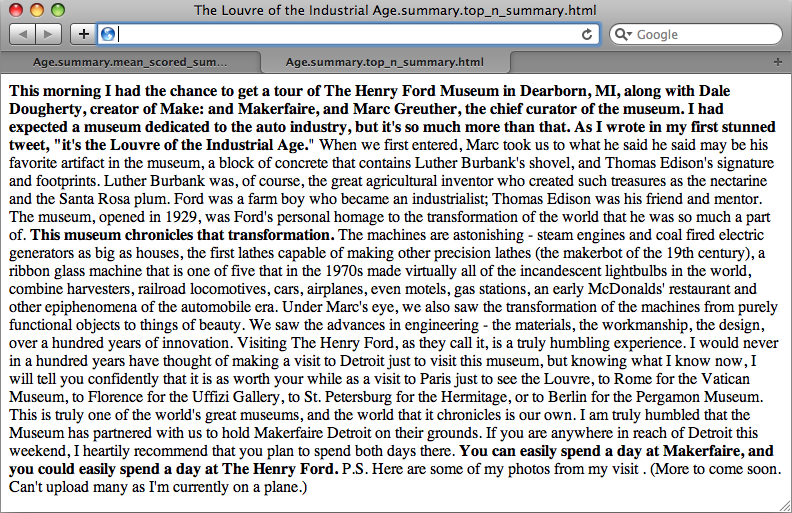
printAs example input/output, we’ll use Tim O’Reilly’s Radar post, “The Louvre of the Industrial Age”. It’s around 460 words long and is reprinted here so that you can compare the sample output from the two summarization attempts in the listing:
This morning I had the chance to get a tour of The Henry Ford Museum in Dearborn, MI, along with Dale Dougherty, creator of Make: and Makerfaire, and Marc Greuther, the chief curator of the museum. I had expected a museum dedicated to the auto industry, but it’s so much more than that. As I wrote in my first stunned tweet, “it’s the Louvre of the Industrial Age.”
When we first entered, Marc took us to what he said may be his favorite artifact in the museum, a block of concrete that contains Luther Burbank’s shovel, and Thomas Edison’s signature and footprints. Luther Burbank was, of course, the great agricultural inventor who created such treasures as the nectarine and the Santa Rosa plum. Ford was a farm boy who became an industrialist; Thomas Edison was his friend and mentor. The museum, opened in 1929, was Ford’s personal homage to the transformation of the world that he was so much a part of. This museum chronicles that transformation.
The machines are astonishing—steam engines and coal-fired electric generators as big as houses, the first lathes capable of making other precision lathes (the makerbot of the 19th century), a ribbon glass machine that is one of five that in the 1970s made virtually all of the incandescent lightbulbs in the world, combine harvesters, railroad locomotives, cars, airplanes, even motels, gas stations, an early McDonalds’ restaurant and other epiphenomena of the automobile era.
Under Marc’s eye, we also saw the transformation of the machines from purely functional objects to things of beauty. We saw the advances in engineering—the materials, the workmanship, the design, over a hundred years of innovation. Visiting The Henry Ford, as they call it, is a truly humbling experience. I would never in a hundred years have thought of making a visit to Detroit just to visit this museum, but knowing what I know now, I will tell you confidently that it is as worth your while as a visit to Paris just to see the Louvre, to Rome for the Vatican Museum, to Florence for the Uffizi Gallery, to St. Petersburg for the Hermitage, or to Berlin for the Pergamon Museum. This is truly one of the world’s great museums, and the world that it chronicles is our own.
I am truly humbled that the Museum has partnered with us to hold Makerfaire Detroit on their grounds. If you are anywhere in reach of Detroit this weekend, I heartily recommend that you plan to spend both days there. You can easily spend a day at Makerfaire, and you could easily spend a day at The Henry Ford. P.S. Here are some of my photos from my visit. (More to come soon. Can’t upload many as I’m currently on a plane.)
Filtering sentences using an average score and standard deviation yields a summary of around 170 words:
This morning I had the chance to get a tour of The Henry Ford Museum in Dearborn, MI, along with Dale Dougherty, creator of Make: and Makerfaire, and Marc Greuther, the chief curator of the museum. I had expected a museum dedicated to the auto industry, but it’s so much more than that. As I wrote in my first stunned tweet, “it’s the Louvre of the Industrial Age. This museum chronicles that transformation. The machines are astonishing - steam engines and coal fired electric generators as big as houses, the first lathes capable of making other precision lathes (the makerbot of the 19th century), a ribbon glass machine that is one of five that in the 1970s made virtually all of the incandescent lightbulbs in the world, combine harvesters, railroad locomotives, cars, airplanes, even motels, gas stations, an early McDonalds’ restaurant and other epiphenomena of the automobile era. You can easily spend a day at Makerfaire, and you could easily spend a day at The Henry Ford.
An alternative summarization approach, which considers only the top N sentences (where N = 5 in this case), produces a slightly more abridged result of around 90 words. It’s even more succinct, but arguably still a pretty informative distillation:
This morning I had the chance to get a tour of The Henry Ford Museum in Dearborn, MI, along with Dale Dougherty, creator of Make: and Makerfaire, and Marc Greuther, the chief curator of the museum. I had expected a museum dedicated to the auto industry, but it’s so much more than that. As I wrote in my first stunned tweet, “it’s the Louvre of the Industrial Age. This museum chronicles that transformation. You can easily spend a day at Makerfaire, and you could easily spend a day at The Henry Ford.
As in any other situation involving analysis, there’s a lot of insight to be gained from visually inspecting the summarizations in relation to the full text. Outputting a simple markup format that can be opened by virtually any web browser is as simple as adjusting the final portion of the script that performs the output to do some string substitution. Example 8-4 illustrates one possibility.
Example 8-4. Augmenting the output of Example 8-3 to produce HTML markup that lends itself to analyzing the summarization algorithm’s results (blogs_and_nlp__summarize_markedup_output.py)
# -*- coding: utf-8 -*-

import os
import sys
import json
import nltk
import numpy
from blogs_and_nlp__summarize import summarize

HTML_TEMPLATE = """<html>
    <head>
        <title>%s</title>
        <meta http-equiv="Content-Type" content="text/html; charset=UTF-8"/>
    </head>
    <body>%s</body>
</html>"""

if __name__ == '__main__':

    # Load in output from blogs_and_nlp__get_feed.py

    BLOG_DATA = sys.argv[1]
    blog_data = json.loads(open(BLOG_DATA).read())

    # Marked up version can be written out to disk

    if not os.path.isdir('out/summarize'):
        os.makedirs('out/summarize')

    for post in blog_data:

        post.update(summarize(post['content']))

        # You could also store a version of the full post with key sentences markedup
        # for analysis with simple string replacement...

        for summary_type in ['top_n_summary', 'mean_scored_summary']:
            post[summary_type + '_marked_up'] = '<p>%s</p>' % (post['content'], )
            for s in post[summary_type]:
                post[summary_type + '_marked_up'] =
                post[summary_type + '_marked_up'].replace(s,
                  '<strong>%s</strong>' % (s, ))

            filename = post['title'] + '.summary.' + summary_type + '.html'
            f = open(os.path.join('out', 'summarize', filename), 'w')
            html = HTML_TEMPLATE % (post['title'] +
              ' Summary', post[summary_type + '_marked_up'],)

            f.write(html.encode('utf-8'))
            f.close()

            print >> sys.stderr, "Data written to", f.name
The resulting output is the full text of the document with sentences comprising the summary highlighted in bold, as displayed in Figure 8-2. As you explore alternative techniques for summarization, a quick glance between browser tabs can give you an intuitive feel for the similarity between the summarization techniques. The primary difference illustrated here is a fairly long (and descriptive) sentence near the middle of the document, beginning with the words “The machines are astonishing”.
The next section presents a brief discussion of Luhn’s approach.
The basic premise behind Luhn’s algorithm is that the important sentences in a document will be the ones that contain frequently occurring words. However, there are a few details worth pointing out. First, not all frequently occurring words are important; generally speaking, stopwords are filler and are hardly ever of interest for analysis. Keep in mind that although we do filter out common stopwords in the sample implementation, it may be possible to create a custom list of stopwords for any given blog or domain with additional a priori knowledge, which might further bolster the strength of this algorithm or any other algorithm that assumes stopwords have been filtered. For example, a blog written exclusively about baseball might so commonly use the word “baseball” that you should consider adding it to a stopword list, even though it’s not a general-purpose stopword. (As a side note, it would be interesting to incorporate TF-IDF into the scoring function for a particular data source as a means of accounting for common words in the parlance of the domain.)
Assuming that a reasonable attempt to eliminate stopwords has been
made, the next step in the algorithm is to choose a reasonable value for
N and choose the top N words
as the basis of analysis. Note that the latent assumption behind this
algorithm is that these top N words are
sufficiently descriptive to characterize the nature of the document, and
that for any two sentences in the document, the sentence that contains
more of these words will be considered more descriptive. All that’s left
after determining the “important words” in the document is to apply a
heuristic to each sentence and filter out some subset of sentences to
use as a summarization or abstract of the document. Scoring each
sentence takes place in the function score_sentences. This is where most of the
interesting action happens in the listing.
In order to score each sentence, the algorithm in score_sentences applies a simple distance
threshold to cluster tokens, and scores each cluster according to the
following formula:
The final score for each sentence is equal to the highest score
for any cluster appearing in the sentence. Let’s consider the high-level
steps involved in score_sentences for an example sentence
to see how this approach works in practice:
- Input: Sample sentence
['Mr.', 'Green', 'killed', 'Colonel', 'Mustard', 'in', 'the', 'study', 'with', 'the', 'candlestick', '.']- Input: List of important words
['Mr.', 'Green', 'Colonel', 'Mustard', 'candlestick']- Input/Assumption: Cluster threshold (distance)
3
- Intermediate Computation: Clusters detected
[ ['Mr.', 'Green', 'killed', 'Colonel', 'Mustard'], ['candlestick'] ]- Intermediate Computation: Cluster scores
[ 3.2, 1 ] # Computation: [ (4*4)/5, (1*1)/1]- Output: Sentence score
3.2 # max([3.2,
              1])
The actual work done in score_sentences is just
bookkeeping to detect the clusters in the sentence. A cluster is defined
as a sequence of words containing two or more important words, where
each important word is within a distance threshold of its nearest
neighbor. While Luhn’s paper suggests a value of 4 or 5 for the distance
threshold, we used a value of 3 for simplicity in this example; thus,
the distance between ‘Green’ and ‘Colonel’ was sufficiently bridged, and
the first cluster detected consisted of the first five words in the
sentence. Note that had the word “study” also appeared in the list of
important words, the entire sentence (except the final punctuation)
would have emerged as a cluster.
Once each sentence has been scored, all that’s left is to determine which sentences to return as a summary. The sample implementation provides two approaches. The first approach uses a statistical threshold to filter out sentences by computing the mean and standard deviation for the scores obtained, while the latter simply returns the top N sentences. Depending on the nature of the data, your mileage will probably vary, but you should be able to tune the parameters to achieve reasonable results with either. One nice thing about using the top N sentences is that you have a pretty good idea about the maximum length of the summary. Using the mean and standard deviation could potentially return more sentences than you’d prefer, if a lot of sentences contain scores that are relatively close to one another.
Luhn’s algorithm is simple to implement and plays to the usual strength of frequently appearing words being descriptive of the overall document. However, keep in mind that like many of the IR approaches we explored in the previous chapter, Luhn’s algorithm makes no attempt to understand the data at a deeper semantic level. It directly computes summarizations as a function of frequently occurring words, and it isn’t terribly sophisticated in how it scores sentences. Still, as was the case with TF-IDF, this makes it all the more amazing that it can perform as well as it seems to perform on randomly selected blog data.
When weighing the pros and cons of implementing a much more complicated approach, it’s worth reflecting on the effort that would be required to improve upon a reasonable summarization such as that produced by Luhn’s algorithm. Sometimes, a crude heuristic is all you really need to accomplish your goal. At other times, however, you may need something more state of the art. The tricky part is computing the cost-benefit analysis of migrating from the crude heuristic to the state-of-the-art solution. Many of us tend to be overly optimistic about the relative effort involved.