
Now that you can (hopefully) better appreciate the nature of the record-matching problem, let’s collect some real-world data from LinkedIn and start hacking out clusters. A few reasons you might be interested in mining your LinkedIn data are because you want to take an honest look at whether your networking skills have been helping you to meet the “right kinds of people,” or because you want to approach contacts who will most likely fit into a certain socioeconomic bracket with a particular kind of business enquiry or proposition. The remainder of this section systematically works through some exercises in clustering your contacts by job title.
An obvious starting point when working with a new data set is to count things, and this situation is no different. This section introduces a pattern for transforming common job titles and then performs a basic frequency analysis.
Assuming you have a reasonable number of exported contacts, the
minor nuances among job titles that you’ll encounter may actually be
surprising, but before we get into that, let’s put together some code
that establishes some patterns for normalizing record data and takes a
basic inventory sorted by frequency. Example 6-2 inspects job titles and prints out
frequency information for the titles themselves and for individual
tokens that occur in them. If you haven’t already, you’ll need to
easy_install pretty table , a
package that you can use to produce nicely formatted tabular
output.
Example 6-2. Standardizing common job titles and computing their frequencies (linkedin__analyze_titles.py)
# -*- coding: utf-8 -*-

import sys
import nltk
import csv
from prettytable import PrettyTable

CSV_FILE = sys.argv[1]

transforms = [
    ('Sr.', 'Senior'),
    ('Sr', 'Senior'),
    ('Jr.', 'Junior'),
    ('Jr', 'Junior'),
    ('CEO', 'Chief Executive Officer'),
    ('COO', 'Chief Operating Officer'),
    ('CTO', 'Chief Technology Officer'),
    ('CFO', 'Chief Finance Officer'),
    ('VP', 'Vice President'),
    ]

csvReader = csv.DictReader(open(CSV_FILE), delimiter=',', quotechar='"')
contacts = [row for row in csvReader]

# Read in a list of titles and split apart
# any combined titles like "President/CEO"
# Other variations could be handled as well such
# as "President & CEO", "President and CEO", etc.

titles = []
for contact in contacts:
    titles.extend([t.strip() for t in contact['Job Title'].split('/')
                  if contact['Job Title'].strip() != ''])

# Replace common/known abbreviations

for i in range(len(titles)):
    for transform in transforms:
        titles[i] = titles[i].replace(*transform)

# Print out a table of titles sorted by frequency

pt = PrettyTable(fields=['Title', 'Freq'])
pt.set_field_align('Title', 'l')
titles_fdist = nltk.FreqDist(titles)
[pt.add_row([title, freq]) for (title, freq) in titles_fdist.items() if freq > 1]
pt.printt()

# Print out a table of tokens sorted by frequency

tokens = []
for title in titles:
    tokens.extend([t.strip(',') for t in title.split()])
pt = PrettyTable(fields=['Token', 'Freq'])
pt.set_field_align('Token', 'l')
tokens_fdist = nltk.FreqDist(tokens)
[pt.add_row([token, freq]) for (token, freq) in tokens_fdist.items() if freq > 1
 and len(token) > 2]
pt.printt()
In short, the code reads in CSV records and makes a mild attempt at normalizing them by splitting apart combined titles that use the forward slash (like a title of “President/CEO”) and replacing known abbreviations. Beyond that, it just displays the results of a frequency distribution of both full job titles and individual tokens contained in the job titles. This is nothing new, but it is useful as a starting template and provides you with some reasonable insight into how the data breaks down. Sample results are shown in Example 6-3.
Example 6-3. Sample results for Example 6-2
+--------------------------+------+
|          Title           | Freq |
+--------------------------+------+
| Chief Executive Officer  |  16  |
| Senior Software Engineer |  12  |
| Owner                    |  9   |
| Software Engineer        |  9   |

...

+-------------+------+
|    Token    | Freq |
+-------------+------+
| Engineer    |  44  |
| Software    |  31  |
| Senior      |  27  |
| Manager     |  26  |
| Chief       |  24  |
| Officer     |  12  |
| Director    |  11  |

...
What’s interesting is that the sample results show that the most common job title based on exact matches is “Chief Executive Officer,” while the most common token in the job titles is “Engineer.” Although “Engineer” is not a constituent token of the most common job title, it does appear in a large number of job titles (for example, “Senior Software Engineer” and “Software Engineer,” which show up near the top of the job titles list). In analyzing job title or address book data, this is precisely the kind of insight that motivates the need for an approximate matching or clustering algorithm. The next section investigates further.
The most substantive decision that needs to be made in taking a set of strings—job titles, in this case—and clustering them in a useful way is which underlying similarity metric to use. There are myriad string similarity metrics available, and choosing the one that’s most appropriate for your situation largely depends on the nature of your objective. A few of the common similarity metrics that might be helpful in comparing job titles follow:
- Edit distance
Edit distance, also known as Levenshtein distance, is a simple measure of how many insertions, deletions, and replacements it would take to convert one string into another. For example, the cost of converting “dad” into “bad” would be one replacement operation and would yield a value of 1. NLTK provides an implementation of edit distance via the
nltk.metrics.distance.edit_distancefunction. Note that the actual edit distance between two strings is often different from the number of operations required to compute the edit distance; computation of edit distance is usually on the order of M*N operations for strings of length M and N.- n-gram similarity
An n-gram is just a terse way of expressing each possible consecutive sequence of n tokens from a text, and it provides the foundational data structure for computing collocations. Peek ahead to Bigram Analysis for an extended discussion of n-grams and collocations.
There are many variations of n-gram similarity, but consider the straightforward case of computing all possible bigrams for the tokens of two strings, and scoring the similarity between the strings by counting the number of common bigrams between them. Example 6-4 demonstrates.
Example 6-4. Using NLTK to compute bigrams in the interpreter
>>>
ceo_bigrams = nltk.bigrams("Chief Executive Officer".split(), pad_right=True,...pad_left=True)>>>ceo_bigrams[(None, 'Chief'), ('Chief', 'Executive'), ('Executive', 'Officer'), ('Officer', None)] >>>cto_bigrams = nltk.bigrams("Chief Technology Officer".split(), pad_right=True,...pad_left=True)>>>cto_bigrams[(None, 'Chief'), ('Chief', 'Technology'), ('Technology', 'Officer'), ('Officer', None)] >>>len(set(ceo_bigrams).intersection(set(cto_bigrams)))2Note that the use of the keyword arguments
pad_rightandpad_leftintentionally allows for leading and trailing tokens to match. The effect of padding is to allow bigrams such as (None, ‘Chief’) to emerge, which are important matches across job titles. NLTK provides a fairly comprehensive array of bigram and trigram scoring functions via theBigramAssociationMeasuresandTrigramAssociationMeasuresclasses defined innltk.metrics.associationmodule.- Jaccard distance
The Jaccard metric expresses the similarity of two sets and is defined by |Set1 intersection Set2/|Set1 union Set2|. In other words, it’s the number of items in common between the two sets divided by the total number of distinct items in the two sets. Peek ahead to How the Collocation Sausage Is Made: Contingency Tables and Scoring Functions for an extended discussion. In general, you’ll compute Jaccard similarity by using n-grams, including unigrams (single tokens), to measure the similarity of two strings. An implementation of Jaccard distance is available at
nltk.metrics.distance.jaccard_distanceand could be implemented as:len(X.union(Y)) - len(X.intersection(Y)))/float(len(X.union(Y))where
XandYare sets of items.- MASI distance
The MASI[41] distance metric is a weighted version of Jaccard similarity that adjusts the score to result in a smaller distance than Jaccard when a partial overlap between sets exists. MASI distance is defined in NLTK as
nltk.metrics.distance.masi_distance, which can be implemented as:1 - float(len(X.intersection(Y)))/float(max(len(X),len(Y)))where
XandYare sets of items. Example 6-5 and the sample results in Table 6-2 provide some data points that may help you better understand this metric.Example 6-5. Using built-in distance metrics from NLTK to compare small sets of items (linkedin__distances.py)
# -*- coding: utf-8 -*-

from nltk.metrics.distance import jaccard_distance, masi_distance
from prettytable import PrettyTable

fields = ['X', 'Y', 'Jaccard(X,Y)', 'MASI(X,Y)']
pt = PrettyTable(fields=fields)
[pt.set_field_align(f, 'l') for f in fields]

for z in range(4):
    X = set()
    for x in range(z, 4):
        Y = set()
        for y in range(1, 3):
            X.add(x)
            Y.add(y)
            pt.add_row([list(X), list(Y), round(jaccard_distance(X, Y), 2),
                       round(masi_distance(X, Y), 2)])
pt.printt()
Notice that whenever the two sets are either completely disjoint or equal—i.e., when one set is totally subsumed[42] by the other—the MASI distance works out to be the same value as the Jaccard distance. However, when the sets overlap only partially, the MASI distance works out to be higher than the Jaccard distance. It’s worth considering whether you think MASI will be more effective than Jaccard distance for the task of scoring two arbitrary job titles and clustering them together if the similarity (distance) between them exceeds a certain threshold. The table of sample results in Table 6-2 tries to help you wrap your head around how MASI compares to plain old Jaccard.
Table 6-2. A comparison of Jaccard and MASI distances for two small sets of items as emitted from Example 6-5
X Y Jaccard (X,Y) MASI (X,Y) [0] [1] 1.0 1.0 [0] [1, 2] 1.0 1.0 [0, 1] [1] 0.5 0.5 [0, 1] [1, 2] 0.67 0.5 [0, 1, 2] [1] 0.67 0.67 [0, 1, 2] [1, 2] 0.33 0.33 [0, 1, 2, 3] [1] 0.75 0.75 [0, 1, 2, 3] [1, 2] 0.5 0.5 [1] [1] 0.0 0.0 [1] [1, 2] 0.5 0.5 [1, 2] [1] 0.5 0.5 [1, 2] [1, 2] 0.0 0.0 [1, 2, 3] [1] 0.67 0.67 [1, 2, 3] [1, 2] 0.33 0.33 [2] [1] 1.0 1.0 [2] [1, 2] 0.5 0.5 [2, 3] [1] 1.0 1.0 [2, 3] [1, 2] 0.67 0.5 [3] [1] 1.0 1.0 [3] [1, 2] 1.0 1.0
While the list of interesting similarity metrics could go on and on, there’s quite literally an ocean of literature about them online, and it’s easy enough to plug in and try out different similarity heuristics once you have a better feel for the data you’re mining. The next section works up a script that clusters job titles using the MASI similarity metric.
Given MASI’s partiality to partially overlapping terms, and that
we have insight suggesting that
overlap in titles is important, let’s try to cluster job titles by
comparing them to one another using MASI distance, as an extension of
Example 6-2. Example 6-6 clusters
similar titles and then displays your contacts accordingly. Take a look
at the code—especially the nested loop invoking the
DISTANCE function that makes a greedy decision—and then
we’ll discuss.
Example 6-6. Clustering job titles using a greedy heuristic (linkedin__cluster_contacts_by_title.py)
# -*- coding: utf-8 -*-

import sys
import csv
from nltk.metrics.distance import masi_distance

CSV_FILE = sys.argv[1]

DISTANCE_THRESHOLD = 0.34
DISTANCE = masi_distance

def cluster_contacts_by_title(csv_file):

    transforms = [
        ('Sr.', 'Senior'),
        ('Sr', 'Senior'),
        ('Jr.', 'Junior'),
        ('Jr', 'Junior'),
        ('CEO', 'Chief Executive Officer'),
        ('COO', 'Chief Operating Officer'),
        ('CTO', 'Chief Technology Officer'),
        ('CFO', 'Chief Finance Officer'),
        ('VP', 'Vice President'),
        ]

    seperators = ['/', 'and', '&']

    csvReader = csv.DictReader(open(csv_file), delimiter=',', quotechar='"')
    contacts = [row for row in csvReader]

# Normalize and/or replace known abbreviations
# and build up list of common titles

    all_titles = []
    for i in range(len(contacts)):
        if contacts[i]['Job Title'] == '':
            contacts[i]['Job Titles'] = ['']
            continue
        titles = [contacts[i]['Job Title']]
        for title in titles:
            for seperator in seperators:
                if title.find(seperator) >= 0:
                    titles.remove(title)
                    titles.extend([title.strip() for title in title.split(seperator)
                                  if title.strip() != ''])

        for transform in transforms:
            titles = [title.replace(*transform) for title in titles]
        contacts[i]['Job Titles'] = titles
        all_titles.extend(titles)

    all_titles = list(set(all_titles))

    clusters = {}
    for title1 in all_titles:
        clusters[title1] = []
        for title2 in all_titles:
            if title2 in clusters[title1] or clusters.has_key(title2) and title1
                in clusters[title2]:
                continue
            distance = DISTANCE(set(title1.split()), set(title2.split()))
            if distance < DISTANCE_THRESHOLD:
                clusters[title1].append(title2)

# Flatten out clusters

    clusters = [clusters[title] for title in clusters if len(clusters[title]) > 1]

# Round up contacts who are in these clusters and group them together

    clustered_contacts = {}
    for cluster in clusters:
        clustered_contacts[tuple(cluster)] = []
        for contact in contacts:
            for title in contact['Job Titles']:
                if title in cluster:
                    clustered_contacts[tuple(cluster)].append('%s %s.'
                            % (contact['First Name'], contact['Last Name'][0]))

    return clustered_contacts

if __name__ == '__main__':
    clustered_contacts = cluster_contacts_by_title(CSV_FILE)

    for titles in clustered_contacts:
        common_titles_heading = 'Common Titles: ' + ', '.join(titles)
        print common_titles_heading

        descriptive_terms = set(titles[0].split())
        for title in titles:
            descriptive_terms.intersection_update(set(title.split()))
        descriptive_terms_heading = 'Descriptive Terms: '
            + ', '.join(descriptive_terms)
        print descriptive_terms_heading
        print '-' * max(len(descriptive_terms_heading), len(common_titles_heading))
        print '
'.join(clustered_contacts[titles])
        print
The code listing starts by separating out combined titles using a list of common conjunctions and then normalizes common titles. Then, a nested loop iterates over all of the titles and clusters them together according to a thresholded MASI similarity metric. This tight loop is where most of the real action happens in the listing: it’s where each title is compared to each other title. If the distance between any two titles as determined by a similarity heuristic is “close enough,” we greedily group them together. In this context, being “greedy” means that the first time we are able to determine that an item might fit in a cluster, we go ahead and assign it without further considering whether there might be a better fit, or making any attempt to account for such a better fit if one appears later. Although incredibly pragmatic, this approach produces very reasonable results. Clearly, the choice of an effective similarity heuristic is critical, but given the nature of the nested loop, the fewer times we have to invoke the scoring function, the better. More will be said about this consideration in the next section, but do note that we do use some conditional logic to try to avoid repeating unnecessary calculations if possible.
The rest of the listing just looks up contacts with a particular job title and groups them for display, but there is one other interesting nuance involved in computing clusters: you often need to assign each cluster a meaningful label. The working implementation computes labels by taking the setwise intersection of terms in the job titles for each cluster, which seems reasonable given that it’s the most obvious common thread. Your mileage is sure to vary with other approaches.
The types of results you might expect from this code are useful in that they group together individuals who are likely to share common responsibilities in their job duties. This information might be useful for a variety of reasons, whether you’re planning an event that includes a “CEO Panel,” trying to figure out who can best help you to make your next career move, or trying to determine whether you are really well-enough connected to other similar professionals given your own job responsibilities. Abridged results for a sample network are presented in Example 6-7.
Example 6-7. Sample output for Example 6-6
Common Titles: Chief Executive Officer,
               Chief Finance Officer,
               Chief Technology Officer,
               Chief Operations Officer
Descriptive Terms: Chief, Officer
----------------------------------------
Gregg P.
Scott S.
Mario G.
Brian F.
Damien K.
Chris A.
Trey B.
Emil E.
Dan M.
Tim E.
John T. H.

...


Common Titles: Consultant,
               Software Engineer,
               Software Engineer
Descriptive Terms: Software, Engineer
-----------------------------------------
Kent L.
Paul C.
Rick C.
James B.
Alex R.
Marco V.
James L.
Bill T.

...It’s important to note that in the worst
case, the nested loop executing the DISTANCE
calculation from Example 6-6 would require it to
be invoked in what we’ve already mentioned is
O(n2) time
complexity—in other words, len(all_titles)*len(all_titles) times. A nested
loop that compares every single item to every single other item for
clustering purposes is not a scalable approach
for a very large value of n, but given that the
unique number of titles for your professional network is not likely to
be very large, it shouldn’t impose a performance constraint. It may
not seem like a big deal—after all, it’s just a nested loop—but the
crux of an O(n2)
algorithm is that the number of comparisons required to process an
input set increases exponentially in proportion to the number of items
in the set. For example, a small input set of 100 job titles would
require only 10,000 scoring operations, while 10,000 job titles would
require 100,000,000 scoring operations. The math doesn’t work out so
well and eventually buckles, even when you have a lot of hardware to
throw at it.
Your initial reaction when faced with what seems like a predicament that scales exponentially will probably be to try to reduce the value of n as much as possible. But most of the time you won’t be able to reduce it enough to make your solution scalable as the size of your input grows, because you still have an O(n2) algorithm. What you really want to do is figure out a way to come up with an algorithm that’s on the order of O(k*n), where k is much smaller than n and represents a manageable amount of overhead that grows much more slowly than the rate of n’s growth. But as with any other engineering decision, there are performance and quality trade-offs to be made in all corners of the real world, and it sure ain’t easy to strike the right balance. In fact, many data-mining companies that have successfully implemented scalable record-matching analytics at a high degree of fidelity consider their specific approaches to be proprietary information (trade secrets), since they result in definite business advantages. (More times than you’d think, it’s not the ability to solve a problem that really matters, but the ability to implement it in a particular manner that can be taken to the market.)
For situations in which an O(n2) algorithm is simply unacceptable, one variation to the working example that you might try is rewriting the nested loops so that a random sample is selected for the scoring function, which would effectively reduce it to O(k*n), if k were the sample size. As the value of the sample size approaches n, however, you’d expect the runtime to begin approaching the O(n2) runtime. Example 6-8 shows how that sampling technique might look in code; the key changes to the previous listing are highlighted in bold. The key takeaway is that for each invocation of the outer loop, we’re executing the inner loop a much smaller, fixed number of times.
Example 6-8. A small modification to an excerpt of Example 6-6 that incorporates random sampling to improve performance
# ...snip ...

all_titles = list(set(all_titles))
clusters = {}
for title1 in all_titles:
    clusters[title1] = []
    for sample in range(SAMPLE_SIZE):
        title2 = all_titles[random.randint(0, len(all_titles)-1)]
        if title2 in clusters[title1] or clusters.has_key(title2) and title1
            in clusters[title2]:
            continue
        distance = DISTANCE(set(title1.split()), set(title2.split()))
        if distance < DISTANCE_THRESHOLD:
        clusters[title1].append(title2)

# ...snip ...
Another approach you might consider is to randomly sample the data into n bins (where n is some number that’s generally less than or equal to the square root of the number of items in your set), perform clustering within each of those individual bins, and then optionally merge the output. For example, if you had one million items, an O(n2) algorithm would take a trillion logical operations, whereas binning the one million items into 1,000 bins containing 1,000 items each and clustering each individual bin would require only a billion operations. (That’s 1,000*1,000 comparisons for each bin for all 1,000 bins.) A billion is still a large number, but it’s three orders of magnitude smaller than a trillion, and that’s nothing to sneeze at.
There are many other approaches in the literature besides sampling or binning that could be far better at reducing the dimensionality of a problem. For example, you’d ideally compare every item in a set, and at the end of the day, the particular technique you’ll end up using to avoid an O(n2) situation for a large value of n will vary based upon real-world constraints and insights you’re likely to gain through experimentation and domain-specific knowledge. As you consider the possibilities, keep in mind that the field of machine learning offers many techniques that are designed to combat exactly these types of scale problems by using various sorts of probabilistic models and sophisticated sampling techniques. The next section introduces a fairly intuitive and well-known clustering algorithm called k-means, which is a general-purpose unsupervised approach for clustering a multidimensional space. We’ll be using this technique later to cluster your contacts by geographic location.
It’s easy to get so caught up in the data-mining techniques themselves that you lose sight of the business case that motivated them in the first place. Simple clustering techniques can create incredibly compelling user experiences (all over the place) by leveraging results even as simple as the job title ones we just produced. Figure 6-2 demonstrates a powerful alternative view of your data via a simple tree widget that could be used as part of a navigation pane or faceted display for filtering search criteria. Assuming that the underlying similarity metrics you’ve chosen have produced meaningful clusters, a simple hierarchical display that presents data in logical groups with a count of the items in each group can streamline the process of finding information, and power intuitive workflows for almost any application where a lot of skimming would otherwise be required to find the results.
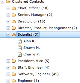
The code to create a simple navigational display can be surprisingly simple, given the maturity of Ajax toolkits and other UI libraries. For example, Example 6-9 shows a simple web page that is all that’s required to populate the Dojo tree widget shown in Figure 6-2 using a makeshift template.
Example 6-9. A template for a Dojo tree widget, as displayed in Figure 6-2—just add data and watch it go!
<!DOCTYPE HTML PUBLIC "-//W3C//DTD HTML 4.01//EN"
		"http://www.w3.org/TR/html4/strict.dtd">
<html>
<head>
	<title>Clustered Contacts</title>
    <link rel="stylesheet"
        href="http://ajax.googleapis.com/ajax/libs/dojo/1.5/dojo/resources/dojo.css">
    <link rel="stylesheet"
        href="http://ajax.googleapis.com/ajax/libs/dojo/1.5/dijit/themes/claro/claro.css">

    <script src="http://ajax.googleapis.com/ajax/libs/dojo/1.5/dojo/dojo.xd.js"
        type="text/javascript" djConfig="parseOnLoad:true"></script>

	<script language="JavaScript" type="text/javascript">
		dojo.require("dojo.data.ItemFileReadStore");
		dojo.require("dijit.Tree");
		dojo.require("dojo.parser");
	</script>

    <script language="JavaScript" type="text/javascript">
        var data = %s; //substituted by Python
    </script>

</head>
<body class="claro">
	<div dojoType="dojo.data.ItemFileReadStore" jsId="jobsStore"
		data="data"></div>

	<div dojoType="dijit.Tree" id="mytree" store="jobsStore"
		label="Clustered Contacts" openOnClick="true">
	</div>
</body>
</html>
The data value that’s substituted into the template
is a simple JSON structure, which we can obtain easily enough by
modifying the output from Example 6-6, as illustrated in
Example 6-10.
Example 6-10. Munging the clustered_contacts data that’s computed in Example 6-6 to produce JSON that’s consumable by Dojo’s tree widget
import json
import webbrowser
import os

data = {"label" : "name", "temp_items" : {}, "items" : []}
for titles in clustered_contacts:
    descriptive_terms = set(titles[0].split())
    for title in titles:
        descriptive_terms.intersection_update(set(title.split()))
    descriptive_terms = ', '.join(descriptive_terms)

    if data['temp_items'].has_key(descriptive_terms):
        data['temp_items'][descriptive_terms].extend([{'name' : cc } for cc
            in clustered_contacts[titles]])
    else:
        data['temp_items'][descriptive_terms] = [{'name' : cc } for cc
            in clustered_contacts[titles]]

for descriptive_terms in data['temp_items']:
    data['items'].append({"name" : "%s (%s)" % (descriptive_terms,
        len(data['temp_items'][descriptive_terms]),),                           "children" : [i for i in
                              data['temp_items'][descriptive_terms]]})

del data['temp_items']

# Open the template and substitute the data

if not os.path.isdir('out'):
    os.mkdir('out')

TEMPLATE = os.path.join(os.getcwd(), '..', 'web_code', 'dojo', 'dojo_tree.html')
OUT = os.path.join('out', 'dojo_tree.html')

t = open(TEMPLATE).read()
f = open(OUT, 'w')
f.write(t % json.dumps(data, indent=4))
f.close()

webbrowser.open("file://" + os.path.join(os.getcwd(), OUT))
There’s incredible value in being able to create user experiences that present data in intuitive ways that power workflows. Something as simple as an intelligently crafted hierarchical display can inadvertently motivate users to spend more time on a site, discover more information than they normally would, and ultimately realize more value in the services the site offers.
Example 6-6 introduced
a greedy approach to clustering, but there are at least two other common
clustering techniques that you should know about: hierarchical
clustering and k-means clustering. Hierarchical
clustering is superficially similar to the greedy heuristic we have been
using, while k-means clustering is radically
different. We’ll primarily focus on k-means
throughout the rest of this chapter, but it’s worthwhile to briefly
introduce the theory behind both of these approaches since you’re very
likely to encounter them during literature review and research. An
excellent implementation of both of these approaches is available via
the cluster module that you can
easy_install, so please go ahead and
take a moment to do that.
Hierarchical clustering is a deterministic and exhaustive technique, in that it computes the full matrix of distances between all items and then walks through the matrix clustering items that meet a minimum distance threshold. It’s hierarchical in that walking over the matrix and clustering items together naturally produces a tree structure that expresses the relative distances between items. In the literature, you may see this technique called agglomerative, because the leaves on the tree represent the items that are being clustered, while nodes in the tree agglomerate these items into clusters.
This technique is similar to but not fundamentally the same as the approach used in Example 6-6, which uses a greedy heuristic to cluster items instead of successively building up a hierarchy. As such, the actual wall clock time (the amount of time it takes for the code to run) for hierarchical clustering may be a bit longer, and you may need to tweak your scoring function and distance threshold. However, the use of dynamic programming and other clever bookkeeping techniques can result in substantial savings in wall clock execution time, depending on the implementation. For example, given that the distance between two items such as job titles is almost certainly going to be symmetric, you should only have to compute one half of the distance matrix instead of the full matrix. Even though the time complexity of the algorithm as a whole is still O(n2), only 0.5*n2 units of work are being performed instead of n2 units of work.
If we were to rewrite Example 6-6 to use the cluster module, the nested loop performing
the clustering DISTANCE computation would be replaced
with something like the code in Example 6-11.
Example 6-11. A minor modification to Example 6-6 that uses cluster.HierarchicalClustering instead of a greedy heuristic (linkedin__cluster_contacts_by_title_hac.py)
# ... snip ...

# Import the goods
from cluster import HierarchicalClustering

# Define a scoring function
def score(title1, title2):
    return DISTANCE(set(title1.split()), set(title2.split()))

# Feed the class your data and the scoring function
hc = HierarchicalClustering(all_titles, score)

# Cluster the data according to a distance threshold
clusters = hc.getlevel(DISTANCE_THRESHOLD)

# Remove singleton clusters
clusters = [c for c in clusters if len(c) > 1]

# ... snip ...
If you’re very interested in variations on hierarchical
clustering, be sure to check out the HierarchicalClustering class’ setLinkageMethod method, which provides some
subtle variations on how the class can compute distances between
clusters. For example, you can specify whether distances between
clusters should be determined by calculating the shortest, longest, or
average distance between any two clusters. Depending on the
distribution of your data, choosing a different linkage method can
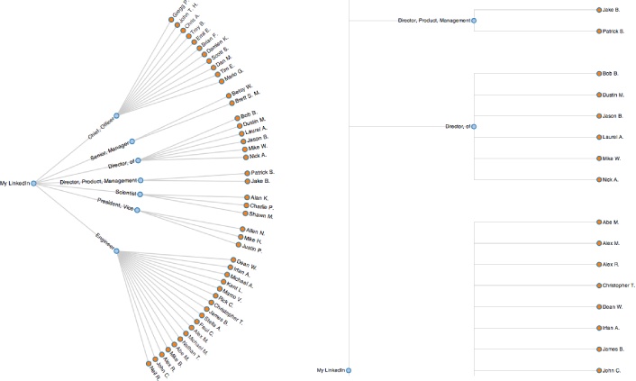
potentially produce quite different results. Figure 6-3 displays a portion of a
professional network as a radial tree layout and a dendogram using
Protovis, a
powerful HTML5-based visualization toolkit. The radial tree
layout is more space-efficient and probably a better choice for this
particular data set, but a dendogram would
be a great choice if you needed to easily find correlations between
each level in the tree (which would correspond to each level of
agglomeration in hierarchical clustering) for a more complex set of
data. Both of the visualizations presented here are essentially just
static incarnations of the interactive tree widget from Figure 6-2. As they show, an amazing amount of
information becomes apparent when you are able to look at a simple
image of your professional network.[43]
Whereas hierarchical clustering is a deterministic technique that exhausts the possibilities and is an O(n2) approach, k-means clustering generally executes on the order of O(k*n) times. The substantial savings in performance come at the expense of results that are approximate, but they still have the potential to be quite good. The idea is that you generally have a multidimensional space containing n points, which you cluster into k clusters through the following series of steps:
Randomly pick k points in the data space as initial values that will be used to compute the k clusters: K1, K2, …, Kk.
Assign each of the n points to a cluster by finding the nearest Kn—effectively creating k clusters and requiring k*n comparisons.
For each of the k clusters, calculate the centroid, or the mean of the cluster, and reassign its Ki value to be that value. (Hence, you’re computing “k-means” during each iteration of the algorithm.)
Repeat steps 2–3 until the members of the clusters do not change between iterations. Generally speaking, relatively few iterations are required for convergence.
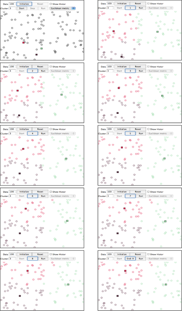
Because k-means may not be all that intuitive at first glance, Figure 6-4 displays each step of the algorithm as presented in the online “Tutorial on Clustering Algorithms”, which features an interactive Java applet. The sample parameters used involve 100 data points and a value of 3 for the parameter k, which means that the algorithm will produce three clusters. The important thing to note at each step is the location of the squares, and which points are included in each of those three clusters as the algorithm progresses. The algorithm only takes nine steps to complete.
Although you could run k-means on points in two dimensions or two thousand dimensions, the most common range is usually somewhere on the order of tens of dimensions, with the most common cases being two or three dimensions. When the dimensionality of the space you’re working in is relatively small, k-means can be an effective clustering technique because it executes fairly quickly and is capable of producing very reasonable results. You do, however, need to pick an appropriate value for k, which is not always obvious. The next section demonstrates how to fetch more extended profile information for your contacts, which bridges this discussion with a follow-up exercise devoted to geographically clustering your professional network by applying k-means.
[41] Measuring Agreement on Set-Valued Items. See http://www.cs.columbia.edu/~becky/pubs/lrec06masi.pdf.
[42] def subsumed(X,Y): return
X.union_update(Y) == X or Y.union_update(X) ==
Y
[43] linkedin__cluster_contacts_by_title_hac.py provides a minimal adaptation of Example 6-6 that demonstrates how to produce output that could be consumed by Protovis.