10
Mixing consoles
![]()
This chapter covers the common mixing (not recording) functionality offered by a typical console. It provides vital background information for Chapter 11, on software mixers, and the chapters succeeding it.
A mixing console (or a desk—both terms are interchangeable) is an independent hardware device used alongside a multitrack recorder at the heart of any recording or mixing session in professional studios. Consoles vary in design, features, and implementation. Products range from compact eight-channel desks through 96-channel large-format analog consoles to large-format digital consoles that can handle more than 500 input signals. In a mixing session, the console’s individual channels are fed with the individual tracks from the multitrack recorder. (It is worth noting the terminology—a channel exists on a console; a track exists on a multitrack recorder.) The mixing console offers three main functionalities:
- Summing—combining the audio signals is the heart of the mixing process; most importantly, various channels are summed to stereo via the mix bus.
- Processing—most consoles have on-board equalizers, while large-format consoles also offer dynamic processors.
- Routing—to enable the use of external processors, effects, and grouping, consoles offer routing functionality in the form of insert points, auxiliary sends, and routing matrices.
All mixing consoles have two distinctive sections:
- Channel section—a collection of channels organized in physical strips. Each channel corresponds to an individual track on the multitrack recorder. The majority of channels on a typical console support a mono input. In many cases, all the channels are identical (functionality and layout), yet on some consoles there might be two or more types of channel strips (for example, mono/stereo channels, channels with different input capabilities, or channels with different equalizers).
- Master section—responsible for central control over the console, and global functionality. For instance, master aux sends, effect returns, control room level, and so on. Large-format analog consoles might also have a computer section that provides automation and recall facilities.
Buses
A bus (or buss in the UK) is a common signal path to which many signals can be mixed. By way of analogy, a bus is like a highway into which many small roads flow. A summing amplifier is an electronic device used to combine (mix) the multiple sources into one signal, which then becomes the bus signal. Most buses are either mono or stereo, but surround consoles also support multichannel buses; for example, a 7.1 mix bus. Typical buses on a large-format console are:
- mix bus;
- group buses (or a single record bus on compact desks);
- auxiliary buses; and
- solo bus.
Processors vs. effects
The devices used to treat audio signals fall into two categories: processors and effects. It is important to understand the differences between the two.
Processors
A processor is a device, electronic circuit, or software code used to alter an input signal and replace i t with the processed, output signal. Processors are used when the original signal is not required after treatment. Processors are therefore connected in series to the signal path (Figure 10.1). If we take an equalizer, for example, it would make no sense to keep the original signal after it had been equalized. Examples of processors include:
- equalizers;
- dynamic range processors;
- compressors;
- limiters;
- gates;
- expanders;
- duckers;
- distortions;
- pitch correctors;
- faders; and
- pan pots.

Figure 10.1 Processors are connected in series to the signal path and replace the original signal with the processed one.
Effects
Effects add something to the original sound. Effects take an input signal and generate a new signal based on that original input. There are then different ways to mix the effect output with the original one. Effects are traditionally connected in parallel with the signal path (Figure 10.2). Most effects are time-based, but pitch-related devices can also fall into this category. Examples of effects include:
- Time-based effects:
- – reverb;
- – delay;
- – chorus; and
- – flanger.
- Pitch-related effects:
- – pitch shifter; and
- – harmonizer.
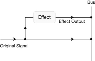
Figure 10.2 In standard operation, a copy of the original signal is sent to an effects unit. The original signal and the effect output are then often mixed when summed to the same bus.
Within an effects unit, we distinguish between two types of signal. The dry signal is simply the unaffected, original input signal. The wet signal is the new signal that the effects unit produces. If we take a delay, for example, the vocal sent to the delay unit makes the dry signal, and the delays generated by the unit constitute the wet signal. While logic has it that effects units should only output the wet signal (and indeed this should be the case when effects are connected in parallel), many effects let us mix internally the dry and wet signals, and output both. The mix between the dry and the wet signal is either determined by a single, percentage-based control, or two separate level controls, one for dry and another for wet (Figure 10.3).
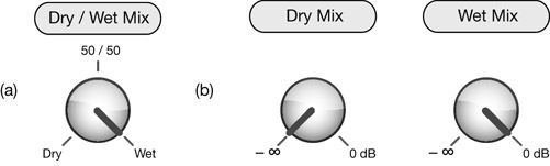
Figure 10.3 Two ways to mix the dry and wet signals within an effect box. (a) A single rotary control with fully dry signal at one extreme, fully wet signal on the other, and equal mix of dry and wet in the center. (b) Two independent controls; each determines the level of its respective signal.
Connecting processors and effects
The standard method for connecting processors is to use an insert point, while effects are normally connected using an auxiliary send. Both are described in detail in this chapter. If processors and effects are not connected as intended, some problems can arise. Still, exceptions always exist; for example, compressors might be connected in parallel as part of the parallel compression technique. In some situations, it makes sense to connect reverbs using inserts. These exceptions are explored in later chapters.
Basic signal flow
In this section, we will use an imaginary six-channel console to demonstrate how audio signals flow within a typical console, and key concepts in signal routing. We will build the console step by step, adding new features each time. Three types of illustrations will be presented in this section: a signal flow diagram, the physical layout of the console, and its rear panel (horizontally mirrored for clarity).
The signal flow diagrams introduced here are schematic drawings that help us understand how signals flow, how these can be routed, and where along the signal path key controls function. By convention, the signal flows from left to right, unless indicated otherwise by arrows. A signal flow diagram is a key part of virtually every console manual. Unfortunately, there isn’t a standard notation for these diagrams, so various manufacturers use different symbols. Common to all these diagrams is that identical sections are shown only once. Therefore, a signal flow diagram of a console with 24 identical channels will only show one channel and this channel is often framed to indicate this. Most master section facilities are unique, and any repetitions are noted (for example, if groups 3–4 function exactly like groups 1–2, the diagram will say “groups 3–4 identical” next to groups 1–2). The signal flow diagrams in this chapter are simplified. For example, they do not include the components converting between balanced and unbalanced.
Step 1: faders, pan pots, and cut switch
The first step involves the basic console shown in Figure 10.4. Each channel is fed from a respective track on the multitrack recorder. As can be seen in Figure 10.4b, each channel has a fader, a pan pot, and a cut switch. The signal flow diagram in Figure 10.4a shows us that the audio signal travels from the line input socket through the cut switch, the fader, and then the pan pot. Each pan pot takes in a mono signal and outputs a stereo signal. The stereo signal is then summed to the mix bus (the summing amplifier is omitted from the illustration) and a single fader alters the overall level of the stereo bus signal. Finally, the mix-bus signal travels to a pair of mono outputs, which reside at the rear panel of the console (Figure 10.4c).
Step 2: line gains, phase-invert, and clip indicators
Many consoles have a line-gain pot, phase-invert switch, and a clip indicator per channel strip. In larger consoles, both the line-gain and phase-invert controls reside in a dedicated input section, which also hosts recording-related controls such as microphone-input selection, phantom power, and a pad switch. Figure 10.5 shows the addition of these controls to our console.
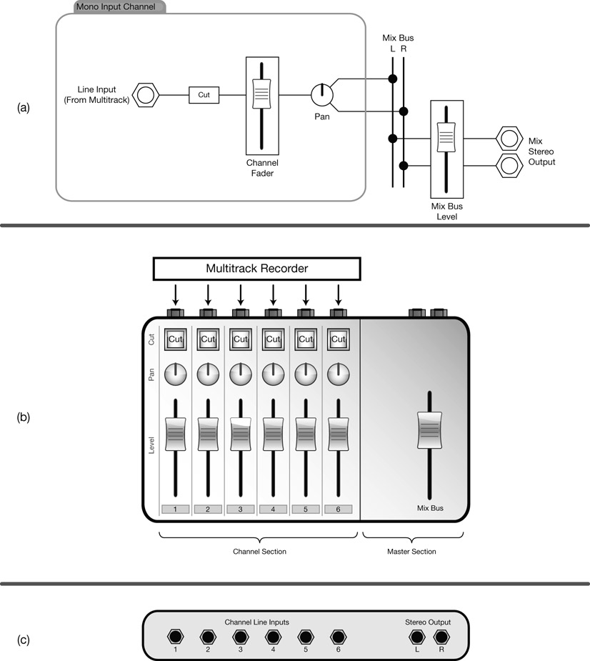
Figure 10.4 The first step in our imaginary six-channel mixer only involves a fader, pan pot, and cut switch per channel. Note that the only control to reside in the master section is the mix-bus level.
The line-gain control (or tape-trim) lets us boost or attenuate the level of the audio signal before it enters the channel signal path. It serves the mixing engineer in two principal ways. First, it lets us optimize the level of the incoming signal. A good recording engineer will make sure that all the tracks on the multitrack recorder are at the optimum level; that is, the highest level possible without clipping (mostly for digital media) or the addition of unwanted distortion (for analog media). If a track level is not optimal, it would be wise to alter it at this early stage. For instance, if the recording level of the vocalist is very low, even the maximum 10 dB extra gain standard faders provide might not be sufficient to make the vocals loud enough in the mix. In such cases, we will need to bring down the rest of the mix, which entails adjusting all other faders. In rare cases, the input signal can be too hot, and might overload the internal channel circuitry. The line-gain pot is used in these situations to bring down the level of the input signal.
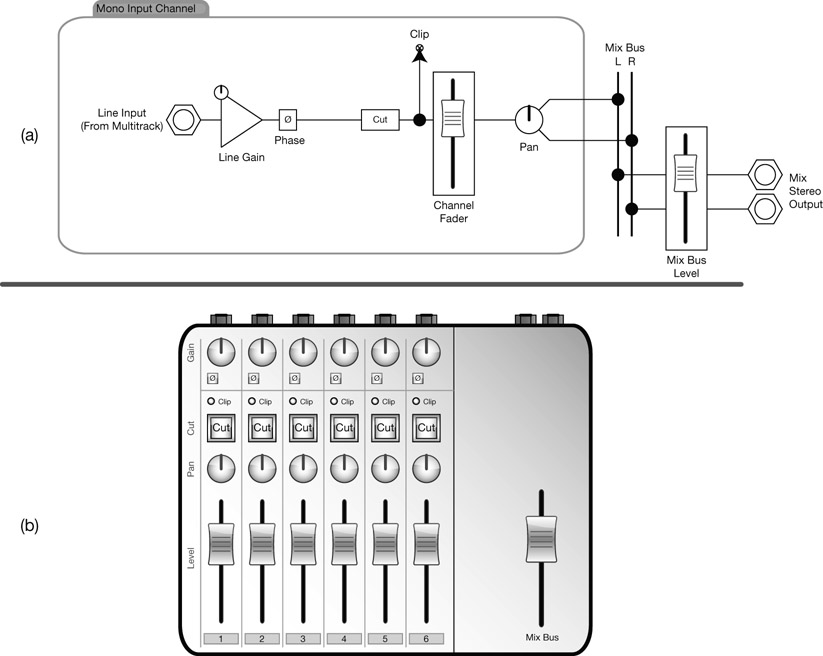
Figure 10.5 In step 2, a line-gain control, a phase-invert switch, and a clip indicator have been added per channel strip. The rear panel of the console is the same as in the previous step and not shown.
Funnily enough, the over-hot input signal is sought after in many situations. An old trick of mixing engineers is to boost the input signal so it intentionally overloads the internal channel circuitry, the reason being that the overloading of the internal analog components is known to produce a distortion that adds harmonics that are quite appealing. Needless to say, it has to be done in the right amounts and on the right instrument. Essentially, the line gain in analog consoles adds distortion capabilities per channel. One thing worth keeping in mind is that dynamic range processors, as well as effect sends, succeed the line-gain stage. Therefore, any line-gain alterations would also require respective adjustment to, for example, the compressor’s threshold or the aux send level. It is therefore wise to set this control during the early stages of the mix, before it can affect other processors or effects in the signal path.
The line-gain controls found on analog consoles are used to add distortion.
A good recording engineer will also ensure that all of the tracks on the multitrack recorder are phase-coherent. In cases where a track was mistakenly recorded with inverted phase, the phase-invert control will make it in-phase.
The clip indicators on an analog console light up when the signal level overshoots a certain threshold set by the manufacturer. There can be various points along the signal path where the signal is tested. The signal flow in Figure 10.5a tells us that in our console, there is only one point before the channel fader. A lit clip indicator on an analog console does not necessarily suggest a sonic impairment, especially if we remember the over-hot signals. If we take some SSL desks, for example, it would not be considered hazardous to have half of the channels clipping when working on a contemporary, powerful mix. The ear should be the sole judge as to whether or not a clipping signal should be dealt with.
Step 3: on-board processors
Most desks offer some on-board processors per channel, from basic tone controls on a compact desk to a filter section, fully featured four-band equalizer, and a dynamics section on large-format consoles. The quality and the number of these on-board processors dictate much of the console’s value, while playing a major role in the console’s sound. Figure 10.6b shows the addition of a high-pass filter, an equalizer, and a basic compressor to each channel on our console. As can be seen in Figure 10.6a, these processors are located in the signal path between the phase and cut stages, as they would appear on a typical console. Some consoles offer dynamic switching of the various processors. For example, a button would switch the dynamics section to before the equalizer.
Step 4: insert points
The on-board processors on a large-format console are known for their high quality, yet in some situations we prefer to use an external unit. Sometimes it is simply because a specific processor is not available on-board (duckers, for example, are not very common, even on large-format consoles), and sometimes the sound of an external device is favored over an on-board processor.
As the name suggests, insertion points let us insert an external device into the signal path. They do so by breaking the signal path, diverting the existing signal to an external device, and routing the returned, externally processed signal so it replaces the original signal. In practice, most consoles always send a copy of the signal to the insert send socket, and the insert button simply determines whether the returned signal is used to replace the existing signal (Figure 10.7). When insert sends are not used to connect an external device, they are used as a place from which a copy of the signal is taken. For example, when adding sub-bass to a kick, a copy of the kick is needed in order to trigger the opening and closing of the gate (more on this in Chapter 19).
It is important to remember that each external unit can only be connected to one specific channel—when using the channel’s insert point, it is impossible to send any other channel to the same external unit. However, it is possible to route the output of one external unit into another external unit and return the output of the latter into the console. This way, we can daisy chain external processors, for example in cases where we want both an external equalizer and a compressor to process the vocal.
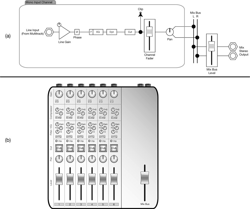
Figure 10.6 As can be seen from the desk layout (b), the additions in step 3 involve a high-pass filter, a singleband fully parametric equalizer, and a basic compressor with threshold, release, and fast attack controls.
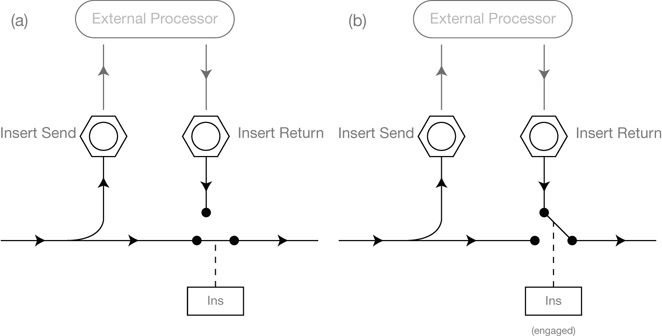
Figure 10.7 A typical insert point. (a) When the insert switch is not engaged, a copy of the signal is still routed to the insert send socket, but it is the original signal that keeps flowing in the signal path. (b) When the insert switch is engaged, the original signal is cut and the insert return signal replaces it.
Figure 10.8a shows the addition of an insert point into our console’s signal flow. Note that the insert point is located after the processors and before the cut stage. Some consoles enable dynamic switching of the insert point, very often before or after the on-board processors. The only addition on the layout itself (Figure 10.8b) is the insert-enable button. On the console’s rear panel in Figure 10.8c, both insert send and return sockets have been added per channel. Two balanced sockets are more common on larger consoles, but some smaller desks utilize one TRS socket that combines both the send (tip) and the return (ring). A Y-lead cable is used in this type of unbalanced connection to connect the external unit.

Figure 10.8 In step 4, insert points have been added to the console per channel. The only addition to the layout (b) is the insert switch, while each channel has additional send and return sockets on the rear panel.
The importance of signal flow diagrams
The console we have designed so far is very typical—both the order of stages in the signal flow and the layout of the controls on the surface are very similar to those of an ordinary console. One thing that stands out immediately is that the controls on the console’s surface are organized for maximum user convenience, and not in the order of processing. Figure 10.9 illustrates how the signal actually travels if we compare it to the channel layout from step 4. We cannot tell just by looking at a desk whether the dynamic processors come before or after the equalizer, tell whether the insert point comes before or after the pro cessors, or gather other signal-flow-related information that can be vital during the mixing process. In many cases, the manual will not answer these questions, leaving the signal flow diagram as our only reference.
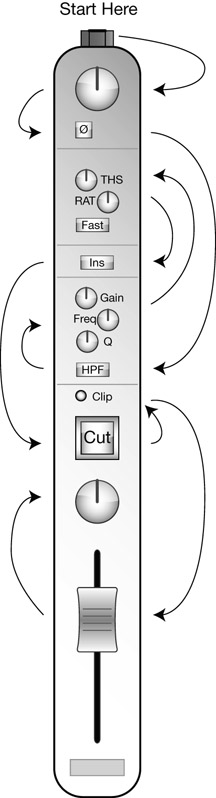
Figure 10.9 This somewhat overwhelming illustration demonstrates how the audio signal really flows through the channel controls.
Step 5: auxiliary sends
An auxiliary send (aux send or send) takes a copy of the signal in the channel path and routes it to an internal auxiliary bus. The auxiliary bus is then routed to an output socket, which could then feed an external effects unit. Each channel strip on the console has a set of aux send-related controls. To distinguish these controls from identical auxiliary controls on the master section, we call them local auxiliary controls; these may consist of:
- Level control—there is always a pot to determine the level of the copy sent to the auxiliary bus.
- Pre-/post-fader switch—a switch to determine whether the signal is taken before or after the channel fader. Clearly, if the signal is taken post-fader, moving the channel fader would alter the level of the sent signal. When connecting effects such as reverbs, we often want the effect level to correspond to the instrument level. Post-fader feed enables this. When the signal is taken pre-fader, its level is independent of the channel fader and will be sent even if the fader is fully down. This is desirable during recording, where the sends determine the level of each instrument in the cue mix—we do not want changes to the monitor mix to affect the artists’ headphone mix. If no switch is provided, the feed can be either pre- or post-fader.
- Pan control—auxiliary buses can be either mono or stereo. When a stereo auxiliary is used, there will be a pan pot to determine how the mono channel signal is panned to the auxiliary bus.
- On/off switch—enables/disables the send to the auxiliary bus. Sometimes simply labeled “mute.”
It is important to understand that we can send each channel to the same auxiliary bus while setting the level of each channel individually using the local aux level (Figure 10.10). For instance, we can send the vocal, acoustic guitar, and tambourine to a single auxiliary bus, which is routed to a reverb unit. With the local aux level controls, we set the level balance between the three instruments, which will eventually result in different amounts of reverb for each instrument. As opposed to insert sends, aux sends allow us to share effects between different channels.
Also, in Figure 10.10, it is worth noting the controls used to set the overall level of the auxiliary bus or cut it altogether. These master aux controls reside in the master section. Master aux controls are often identical to the local ones, with one exception: there is never a pre-/post-fader control. These are done on a per channel basis and not globally for each auxiliary bus.
Most consoles have more than one auxiliary bus, and thus more than one set of local and master aux controls. On some consoles, the number of auxiliaries determines how many effects units can be used in the mix. For example, in a console with only two auxiliaries, aux 1 might be routed to a reverb unit, with aux 2 to a delay unit. As with inserts, we can daisy chain units in order; for example, to have aux 1 sent to a delay, which is then followed by a reverb. The different aux sends are not always identical, and each might involve a slightly different set of controls. In the case of our console, two aux sends have been added (Figure 10.11). Aux 1 is stereo, has a pre-/post-switch, pan control, and a cut switch. Aux 2 is mono and only features level and cut controls. As can be seen in Figure 10.11a, aux 1 has a fixed post-fader feed. To the desk layout in Figure 10.11b, the respective controls for each local aux have been added per channel. Also, the master section now offers both level and cut controls for each master aux. Figure 10.11c shows the addition of output sockets per auxiliary.
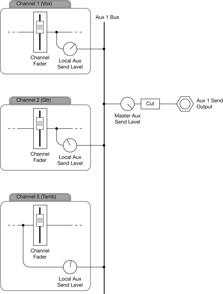
Figure 10.10 In this illustration, the signals from three channels are sent to the same auxiliary bus, each with its own send level settings. Note that for channels 1 and 2, a post-fader feed is selected, while for channel 5 there is a pre-fader feed.


Figure 10.11 In step 5, auxiliary sends were added. The console has two auxiliary buses, one stereo and the other mono. As per channel, the local controls for aux send 1 are level, pre-/post-fader selection, pan, and cut. Aux 2 only has local level and cut controls. The master aux controls for both auxiliaries are level and cut.
Step 6: FX returns
So far, we have seen how we can send an audio signal to an effects unit. Let us consider now how the effect return can be brought back to the console. FX returns (sometimes called aux returns) are dedicated stereo inputs at the back of the desk that can be routed to the mix bus. All but the most basic desks provide some master controls to manipulate the returned effect signal. Level and mute are very common, while large-format desks might also have some basic tone controls. Figure 10.12 shows the addition of two stereo FX returns to our desk. In the layout in Figure 10.12b, a dedicated section provides level and mute controls for each return, and two pairs of additional sockets have been added to the rear panel in Figure 10.12c.
FX returns provide a very quick and easy way to blend an effect return into the mix, but even on large-format consoles they offer very limited functionality. For example, they rarely let us pan the returned signal, which might be needed in order to narrow down the width of a stereo reverb return. As an alternative, mixing engineers often return effects into two mono channels, which offer greater variety of processing (individual pan pots, equalizers, compressors, etc.). Such a setup is shown in Figure 10.13.
When possible, effects are better returned into channels.
Groups
Rarely do raw tracks not involve some logical groups. The individual drum tracks are a prime example of a group that exists in most recorded productions; vocals, strings, and guitars are also potential groups. While a drum group might consist of 16 individual tracks, some groups might only consist of two—bass-mic and bass-direct, for example. During mixdown, we often want to change the level of, mute, solo, or process collectively a group of channels. The group facility allows us to do so. There are two types of groups: control and audio.
Control grouping
Control grouping is straightforward. We first allocate a set of channels to a group, so that moving one fader causes all the other faders in the group to move simultaneously. Cutting or soloing a channel also cuts or solos all other group channels. Some consoles define this behavior as linking, while grouping denotes a master–slave relationship—only changes to the master channel result in respective changes to the slaves, but changes to slaves do not affect other channels.
VCA grouping
VCA grouping is an alternative type of control grouping. In order for faders to respond to the movement of other faders, they must be motorized. Consoles without motorized faders can achieve something similar using a facility called VCA grouping. With VCA grouping, a set of master VCA group faders are located in the master section alongside the cut and solo buttons per group. Individual channel faders can then be assigned to a VCA group using a dedicated control per channel strip. Moving a master VCA group fader alters the
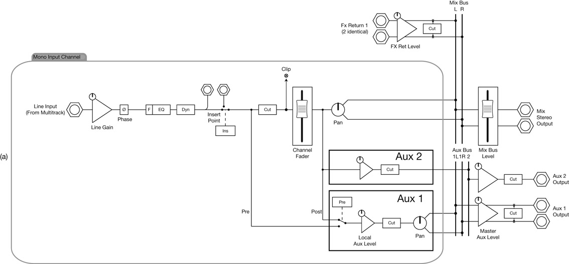

Figure 10.12 Step 6 involves the addition of two FX returns. There are two pairs of sockets on the rear panel; each FX return has level and cut controls that will affect the returned effect signal before it is summed to the mix bus.

Figure 10.13 When there are free channels on the console, mixing engineers often bring back effect returns into channels rather than using FX returns. Channels offer more processing options compared to FX returns.
level of all channels assigned to the VCA group (the channel faders will not physically move). Cutting or soloing a VCA group cuts or solos all the assigned channels. Figure 10.14 shows the layout of a small console with VCA groups.
![]()
The concept of VCA faders is explained in Chapter 13.
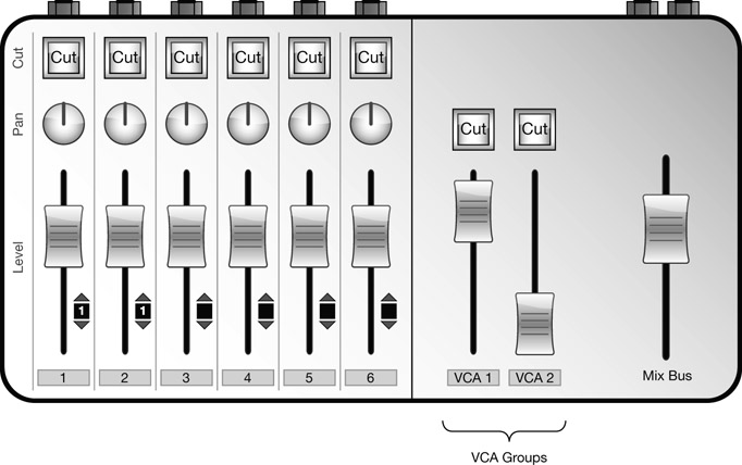
Figure 10.14 A basic console with two VCA groups. In the illustration above, channels 1 and 2 are assigned to VCA group 1. Moving the fader of VCA group 1 will alter the level of channels 1 and 2, although their faders will not move.
Control grouping is great when we want to control collectively a group of channels. In addition to the standard level, cut, and solo controls, digital consoles (and software mixers) sometimes enable the grouping of additional controls such as pan pots, aux sends, or the phase-invert switches. However, control grouping does not alter the original signal path; therefore, it is impossible to process a group of channels collectively. This is often required; for example, in cases where we want to compress the overall drum mix. When collective processing is needed or if an analog console does not offer control grouping, audio grouping is the solution.
Audio grouping
To handle many signals collectively, a group of channels must first be summed to a group bus—a practice called subgrouping. The group signal (essentially a submix) can then be processed and routed to the mix bus. Different consoles provide different numbers of group buses, with multiples of eight being the most common. Each group bus is mono, but very often groups are used in stereo pairs made of consecutive odd and even groups—each represents left and right, respectively. For example, in groups 1–2, group 1 is left and 2 is right. The format Channels:Groups:Mix-Buses is commonly used to describe the number of these facilities on a console. For example, 16:8:2 denotes 16 channels, eight group buses, and two mix buses (i.e., one stereo mix bus).

Figure 10.15 Routing matrices. (a) A typical arrangement for a routing matrix on a large console. Each group bus has a dedicated button. (b) A typical arrangement for a routing matrix on a smaller desk. Each button assigns the channel signal to a pair of groups, and the channel pan pot can determine to which of the two the signal is sent.
Each channel can be assigned to different groups using a routing matrix that resides on each channel strip. A routing matrix is a collection of buttons that can be situated either vertically next to the fader or in a dedicated area on the channel strip (Figure 10.15), the latter being more common on larger desks, where there can be up to 48 groups. Routing matrices come in two formats—those that have an independent button for each group bus and those that have a button for each pair of groups. A pan pot usually determines how the signal is panned when sent to a pair of groups. For example, if groups 1 and 2 are selected and the pan pot is turned hard-left, the signal will only be sent to group 1.
As far as the signal flow goes, the signal sent to the group is a copy of the channel signal. We need a way to disconnect the original signal from the mix bus, since the copy sent to the group will be routed to the mix bus anyway (seldom do we want both the original and the copy together on the mix bus). To achieve this, each routing matrix has a mix assignment switch that determines whether or not the original channel signal feeds the mix bus. The copy is taken post the channel pan pot (and thus post the channel fader), and therefore any processing applied to the channel signal (including fader movements) affects the copy sent to the group. It should be made clear that with audio grouping, we have full processing control over each individual channel and on the group itself. We can, for example, apply specific compression to the kick, different compression to the snare, and different compression still to the drum mix.
Group facilities fall into two categories: master groups and in-line groups. Consoles that offer master groups provide a dedicated strip of controls for each group bus on the master section. Each strip contains a fader that sets the overall level of the group, and a few additional controls such as a solo button or a mix-bus assignment switch. The latter is required, as during recording or bouncing the group buses are not normally assigned to the mix bus. The mix-bus assignment switch also acts as a mute control since it can disconnect the group signal from the mix bus. To enable the processing of the group signal, each group offers an insertion point.
Figure 10.16a shows the signal flow of a console with master audio groups. Note that the signal to the group bus is a copy taken post-pan. Each group has an insert point (in this case half-normalled, like on a standard patchbay), a fader, and a mix-bus assignment switch. With this console, odd groups can only be assigned to the left, and even groups to the right—effectively forcing the groups to work as stereo pairs. Most consoles also have a button to assign each group to both channels of the mix bus. In Figure 10.16b, we can see the routing matrix next to each channel fader, which involves an assignment button to the mix bus and to each pair of groups. There are also four master group strips; each contains a fader and an assignment switch to either the left or right mix buses. Figure 10.16c shows the addition of the group insert sockets to the rear of the console.
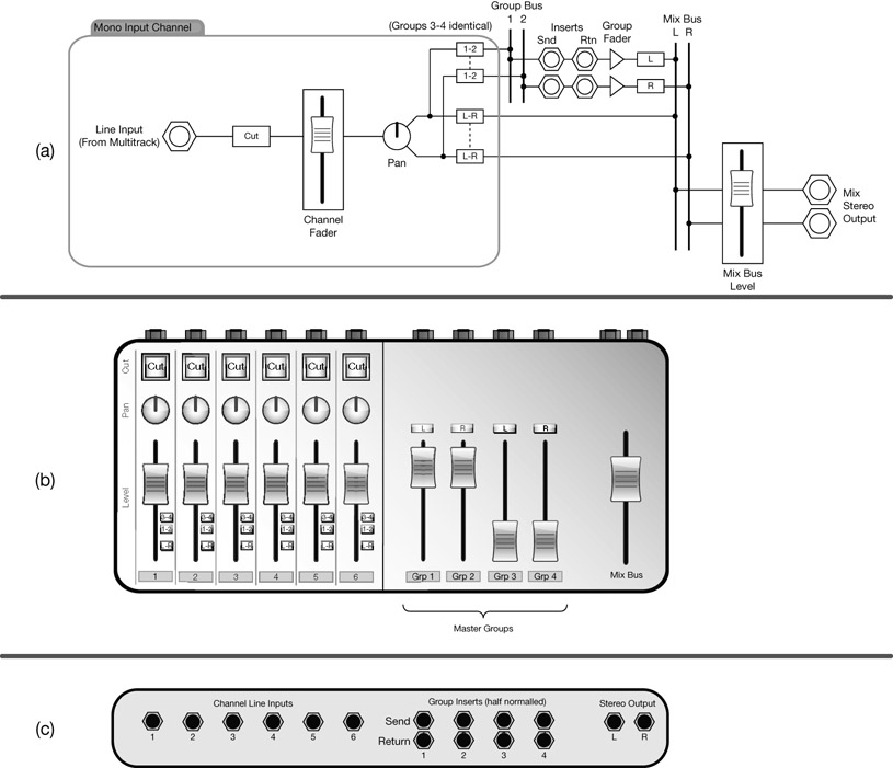
Figure 10.16 A basic console with four master audio groups. In this illustration, channels 1–2 are assigned to groups 1–2; the rest of the channels are assigned to the mix bus and so are groups 1–2.
In-line groups are only found on large-format in-line desks. These desks still have a routing matrix per channel, but they do not offer any master group strips. Instead, each channel strip hosts its associated group (for instance, channel 1 hosts group 1, channel 2 hosts group 2, and so forth). Once hosted, the group signal is affected by all the channel components, including the fader, pan pot, on-board equalizer, compressor, and insert point. These provide much more functionality than any master group might. But this functionality comes at a price—each channel can only be used to either handle a track from the multitrack

Figure 10.17 Basic schematic of audio groups. Channels 1–8 are routed to groups 25–26, which are then fed into their associated channels.

Figure 10.18 A console with in-line group facilities. Channels 1–3 are routed to groups 5–6. The pressed group buttons on channels 5–6 bring the group signal into these channels, which are the only ones assigned to the mix bus.
or host its associated group; it cannot do both. In order to use in-line groups, we must have more channels than tracks. On most large consoles, this is not an issue—if the multitrack has 24 tracks, they will feed channels 1–24, while channels 25–48 will be available as in-line groups. A possible scenario would involve disconnecting all the drum channels (say, 1–8) from the mix bus and routing them to groups 25–26. Channels 25–26 would then be used to host groups 25–26. To route the two groups to the mix bus, all we would need to do is select the mix bus on the routing matrices of the hosting channels (Figure 10.17).
A group button on the input section of each channel determines what signal feeds the channel path: either the multitrack return signal (the track coming back from the multitrack via the line input) or the associated group signal (which turns the channel into its associated group host). In the case of the drum scenario illustrated above, it will be pressed on channels 25 and 26. Pressing the group button on a channel that has its associated group selected on the routing matrix will cause feedback (the channel will be routed to the same group that feeds it).
Figure 10.18 illustrates a hypothetical desk, as it involves in-line groups on a split desk. Yet it demonstrates well the concept of audio groups. The signal flow in Figure 10.18 shows that pressing the group button will feed the associated group signal into the channel path before the phase button. All the groups in this case are just being sent back to their associated channels. Figure 10.18b reveals a dedicated routing matrix per channel with an assignment button per group (and one button for the mix bus). Also, the group button was added next to the phase button.
Bouncing
The concept of bouncing is explained in Appendix A. So far, we have only discussed groups in relation to mixing, but groups are an essential part of the recording process as they provide the facility to route incoming microphone signals to the multitrack recorder. Every console that offers group buses also has an output socket per group bus. The group outputs are either hardwired or can be patched to the track inputs of the multitrack recorder. The process of bouncing is similar to the process of recording, except that instead of recording microphone signals, we record a submix. In order to bounce something, all we have to do is route the channels of our submix to a group and make sure that the group output is sent to an available track on the multitrack recorder. Since most submixes are stereo, this process usually involves a pair of groups.
Figure 10.19 shows the console in Figure 10.18 but with the additional group outputs. If you remember, the less-than-optimum level is one of the most common issues with bouncing, and setting the group level is one way to bring the bounced signal to its optimal level. Figure 10.19a shows that the group signal ends up in a group output socket, but only after it has passed a level control. One question that might arise is: Where exactly on the desk do we put these group-level controls? We could place them on the master section, but since consoles with in-line groups have as many groups as channels (commonly up to 48 groups) and since these channels and groups are associated, it makes sense to put the group level on each channel strip. As can be seen in Figure 10.19b, the group-level control has been added just below the group button. Figure 10.19c illustrates the addition of the group output sockets, as expected, aligned with the channel inputs.

Figure 10.19 A console with physical group outputs, and group-level controls.
In-line consoles
The recording aspects
It is impossible to discuss the merits of in-line consoles without talking about recording, but discussion of the latter will be kept brief. During a recording session, the desk accommodates two types of signal: (a) the live performance signals, which are sent via the groups to be recorded on the multitrack; and (b) the multitrack return signals, which include any previously recorded instruments. On a split desk, which we have discussed so far, some channels handle the live signals while others handle the multitrack return signals. But a single channel cannot handle two signals at the same time. Figure 10.20 shows the layout of a split desk during recording.

Figure 10.20 An eight-channel, four-group desk as might be utilized in a recording situation. Channels 1–4 will handle live signals coming through the microphone or line inputs, channels 5–8 will handle the signals returning from the multitrack via the line inputs, and the master group will be used to route the incoming signals to the multitrack.
Split designs can be large. For example, a 24-track recording would require a 48-channel console—24 channels for live signals and 24 for multitrack returns. If the console also includes 24 master groups, we end up with 72 strips. Size aside, each channel strip costs a good amount of money. However, we rarely require all the expensive features on all channels—we either process the live signals or the multitrack return signals, seldom both.
Going in-line

Figure 10.21 The SSL 4000 G+. This photo clearly shows the two faders per I/O module. Depending on the desk configuration, one fader controls the level of the monitor path, the other the channel path.
Source: Courtesy of SAE, London.
The way in-line designs solve the size issue is by squeezing 48 channels into 24 I/O modules (referred to as channel strips on a split desk). This is done by introducing additional signal path to the existing channel path on each I/O module. While the channel path is used for live signals, the new path is used for multitrack return signals. Since it is the latter that we monitor (both in the control room and in the live room), the new path is called the monitor path. The additional requirements for each I/O module include a line input socket for the multitrack return signal and a fader (or pot on smaller desks) to control the level of the monitor path signal. Large in-line consoles are easily identified by the two faders that reside on each I/O module (Figure 10.21). There will still be only one equalizer, compressor, aux send, and insert point per I/O module, but each facility can be switched to either the channel or monitor path (console permitting).
So we can condense a 48-channel split desk into a 24-channel in-line desk, but what about the additional 24 master groups? If we exchange them for 24 in-line groups (as in Figure 10.18), we can integrate those groups into our 24 I/O modules. We will then end up with 24 I/O modules, each with a channel path, monitor path, and a group, all in-line (Figure 10.22).
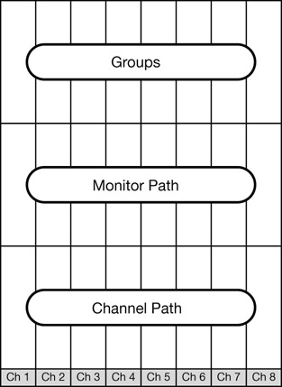
Figure 10.22 An eight-channel in-line console.
A 24-track studio might benefit from the in-line concept, but if the studio has a small live room—where only eight microphones may be used simultaneously—it would only need eight groups on its console. A specific design combines a channel and monitor path per I/O module, with master instead of in-line groups. Figure 10.23 illustrates this concept, while Figure 10.24 shows such a console.
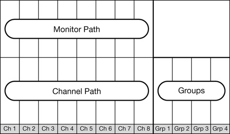
Figure 10.23 An eight-channel, four-group console.

Figure 10.24 The Mackie Analog 8-Bus. Each I/O module has separate level and pan controls per path. In the case of the 8-Bus, the level of one path is controlled using a fader, while the level of the other is controlled using a pot (the white row left of the meters). The eight master group faders can be seen on the right (between the channel faders and master fader).
In-line consoles and mixing
The in-line design makes consoles smaller and cheaper, but as effective for recording. When it comes to mixing, they make things slightly more complex than the split design. The first thing to understand is that a 24-channel console is able to accommodate 48 input signals as each I/O module has both channel and monitor paths. In a 24-track studio, this means the addition of 24 free signal paths during mixdown. As already mentioned, the different processing and routing facilities can only be switched to one path at a time. The catch is that not all facilities can be switched to the monitor path—the insert point, for example, might be fixed on the channel path. Generally, the channel path is the “stronger” path—providing full functionality—while the monitor path is more limited. It is therefore reasonable to use the channel path for the main mix of multitrack return signals and utilize the monitor path for a variety of purposes. Under normal circumstances, the monitor path is used for the following:
- Effect returns—effect returns can be easily patched to the monitor path via its line input. We can, for example, send a guitar from the channel path to a delay unit and bring the delay back to the monitor path on the same I/O module.
- Additional auxiliary sends—even the most respectable large-format consoles can be limited to five auxiliaries, only one of which might be stereo. While this is sufficient for recording, it can restrict effect usage during mixdown—what if we need more than five effects? By having a copy of the channel signal in the monitor path, we can route it to a group, which is then routed to an effects unit. In this scenario, the monitor path level control acts as a local aux send, while the group level acts as master auxiliary level.
- Signal copies—in various mixing scenarios, a signal duplicate is needed and the monitor path is the native host for these duplicates. One example is the parallel compression technique.
The monitor section
In addition to the global sections we have covered so far, the master section may also contain subsections dealing with global configuration, monitoring, metering, solos, cue mix, and talkback. Out of these, the monitor section is the most relevant for mixdown. Needless to say, the selection of features is dependent on the actual make. The following section is limited to the most common and useful features.
The monitor output
The imaginary console we have built so far has had a stereo mix output all along. The mix output, conventionally, only outputs the mix-bus signal and should be connected to a two-track recorder. Although most of the time we monitor the mix bus, sometimes we want to listen to an external input from a CD player, a soloed signal, an aux bus, or some other signals. To enable this, consoles offer monitor output sockets, which, as you might guess, are connected to the monitors. There is also a separate gain control, usually a pot, to control the overall monitoring level.
Figure 10.25 shows the addition of the monitor output facilities to the basic console in step 1. In Figure 10.25a, both the mix bus and an external input (2TK input or two-track input) are connected to the monitor output. A control circuit cuts all the inactive monitor alternatives. The monitor gain is determined by the CR Level pot (control room level). It is worth noting that the mix level will affect the monitor level, but not the other way around. This lets us alter the monitor level without changing the signal level sent to a two-track recorder via the mix output. If we want to fade our mix, we must use the mix level. Figure 10.25b illustrates the addition of the monitor gain control, labeled “monitor level.” At the rear of the desk in Figure 10.25c, a pair of monitor output sockets have been added, as well as a pair of external input sockets.
Additional controls
Figure 10.26 illustrates a master monitor section, very similar to that found on a large-format console. The various controls are:
- Cut—cuts the monitor output. Used in emergencies, such as sudden feedback or noise bursts. Also used to protect the monitors from predictable clicks and thumps caused by computers being turned on and off, or patching.
- Dim—attenuates the monitor level by a fixed number of dBs, which is sometimes determined by a separate pot (around 18 dB is common). The monitor output will still be audible, but at a level that enables easier communication between people in the room or on the other end of a telephone.
- Mono—sums the stereo output into mono. Enables mono-coherence checks and can be used as an aid when dealing with masking.
- Speaker selection—a set of buttons for switching between the different sets of loudspeakers; that is, the full-range, near-fields, and mini-speakers. It is also possible to have an independent switch that toggles the subwoofer on and off. A console with such a facility will have individual outputs for each set of speakers.
- Cut left, cut right—two switches: each cuts its respective output channel. Used during mix analysis and to identify suspected stereo problems, for example a reverb missing from the left channel due to a faulty patch lead.
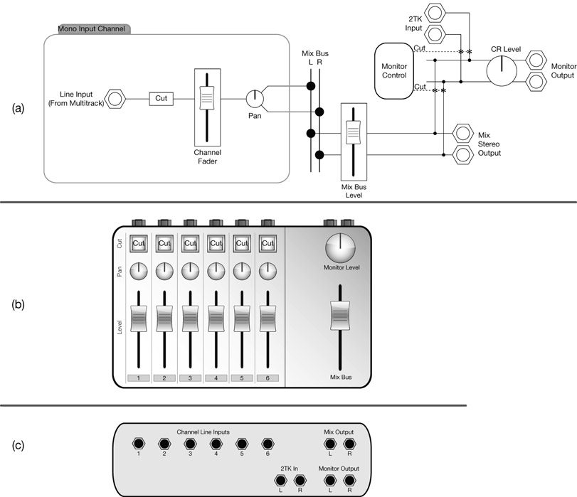
Figure 10.25 A basic console with monitor output facilities.
- Swap left/right—swaps the left and right monitor channels. Swapping the mix channels can be disturbing since we are so used to the original panning scheme. Also, in a room with acoustic stereo issues (due to asymmetry, for example), pressing this button can result in altered tonal and level balances, which are even more disturbing. This button is used to check stereo imbalance in the mix. If there is such an imbalance, pressing this button might make us feel like turning our head toward one of the speakers; if it is unclear toward which speaker the head should turn, the stereo image is likely to be balanced. Image shifting can also be the result of problems in the monitoring system, such as when the vocals are panned center but appear to come from an off-center position. If by pressing this button the vocals remain at the same off-center position, one speaker might be louder than the other or one of the speaker cables (or amplifier channels) might be attenuating the channel signal. If the vocal position is mirrored around the center, then it is clear that the shifting is part of the mix itself.
- Source selection—determines what feeds the monitor outputs. Sources might include the mix bus, external inputs, or an aux bus. Sources might be divided into internal and external sources, and additional controls let us toggle between the two types.
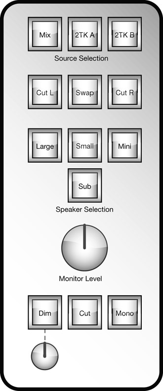
Figure 10.26 A master monitor section.
Solos
Solo modes determine how the solo facility operates; that is, what exactly happens when a channel is soloed. There are two principal types of solo: destructive and nondestructive. Nondestructive solos can be PFL, AFL, or APL (the meanings of which will be covered shortly). The hierarchy of the different solo modes is as follows:
- destructive in-place; and
- nondestructive:
- – PFL; and
- – AFL or APL.
Large consoles often support more than one type of solo mode; for example, a desk might support destructive solo, PFL, and APL. A console can either support AFL or APL solo, but rarely both. Often manufacturers use the term AFL for a facility that is essentially APL.
The active solo mode can be selected through a set of switches that reside on the master section. In certain circumstances (discussed soon), a desk will toggle momentarily to nondestructive mode.
Destructive solo
Destructive solo might also be called in-place, destructive in-place, mixdown solo, or SIP, which stands for solo in-place. In destructive solo mode (Figure 10.27), whenever a channel is soloed all the other channels are cut. Therefore, only the soloed channel (or channels) is sent to the mix bus (which is still monitored). It should be clear that both channel level and panning information are maintained with this type of solo.
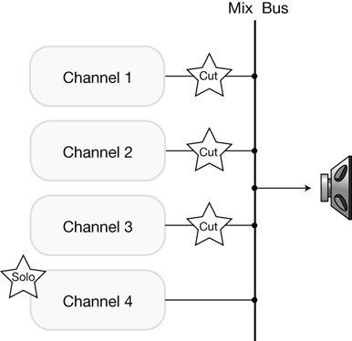
Figure 10.27 Destructive in-place solo. (It is worth knowing that in practice the individual channels are cut by internal engagement of their cut switch.)
Nondestructive solo
In nondestructive mode (Figure 10.28), no channel is being cut. Instead, the soloed channels are routed to a solo bus. As long as solo is engaged, the console automatically routes the solo bus to the monitors, cutting momentarily the existing monitor source (normally the mix bus). With nondestructive solo, the mix output remains intact as all the channels are still summed to the mix bus. PFL (pre-fade listen), AFL (after-fade listen), and APL (after-pan listen) signify the point along the channel signal path from which the signal is taken (Figure 10.29). PFL takes a copy before the channel fader and pan pot; therefore, both mix levels and panning are ignored. AFL takes a copy after the fader but before pan, so it maintains mix levels but ignores panning. APL takes a copy after both fader and pan, so both level and panning are maintained. Only a desk that provides APL solo requires a stereo solo bus; for PFL and AFL solos, a mono bus will suffice.
A solo-bus level control is provided on the master section. It is recommended to set this control so that signals are neither boosted nor attenuated once soloed. Essentially, this involves leveling the solo bus with the mix-bus level. Any other setting and the mixing engineer might be tempted to approach the monitor level following soloing; then, when solo is disengaged, the monitored mix level will either drop or rise, which might again lead to alteration of the monitor level. The greatest danger of this is constantly rising monitor levels.
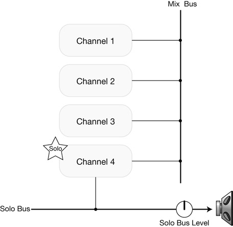
Figure 10.28 Nondestructive solo.
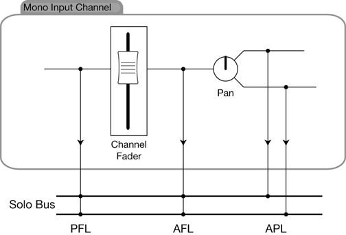
Figure 10.29 Depending on the console and the global solo mode, soloed signals can be sourced from one of three different points along the channel path.
Solo safe
Solo safe (or solo isolate) provides a remedy to problems that arise as part of the destructive solo mechanism. More specifically, it prevents channels flagged as solo safe from being cut when another channel is soloed. A good example of channels that should be solo safe would be those hosting an audio group. If soloing a kick subsequently cuts the drum group to which it is routed, the monitors output null (Figure 10.30a). To prevent them from being cut, the channels hosting the drum group are flagged as solo safe. The same null can occur if the audio group channels are soloed since this will cut the source channels, including the kick (Figure 10.30b). Unfortunately, a console cannot determine the individual source channels of an audio group, so in order to prevent them from being cut the console would automatically engage into nondestructive solo mode when solosafe channels are soloed. Along with audio groups, effect returns are also commonly flagged as solo safe.

Figure 10.30 Two problematic scenarios with destructive solos and audio grouping. (a) Soloing a source channel will cut the group it is routed to. (b) Soloing the group hosting channels will cut the source channels.
Which solo?
Destructive solo is considered unsafe during recording. Recording during mixdown only happens in two situations: when we bounce and when we commit our mix to a two-track recorder. In these cases, any destructive solo will be imprinted on the recording, which is seldom our intention. With the exception of this risk, destructive solo offers many advantages over nondestructive solo. First, if the console involves a mono solo bus, all soloed signals are monitored in mono. This is highly undesirable, especially for stereo tracks and effect returns (e.g., overheads or stereo reverb). With destructive solo, we listen to the stereo mix bus, so panning information is maintained. Another issue with non destructive solo has to do with unwanted signals on effect returns. Consider a mix where both the snare and the organ are sent to the same reverb unit, and in order to work on the snare and its reverb we solo both. In this scenario, the reverb return still carries the organ reverb, since nothing prevents the organ from feeding its aux send. By soloing in destructive mode, the organ channel will be cut and so will its aux feed to the reverb. Destructive solo also ensures that the soloed signal level remains exactly as it was before soloing. In nondestructive solo, soloed signals might drop or rise in level, depending on the level of the solo bus.
Destructive solo is favored for mixdown.
The only time PFL solo comes in handy during mixdown is when we want to audition the multitrack material with faders down.
Correct gain structure
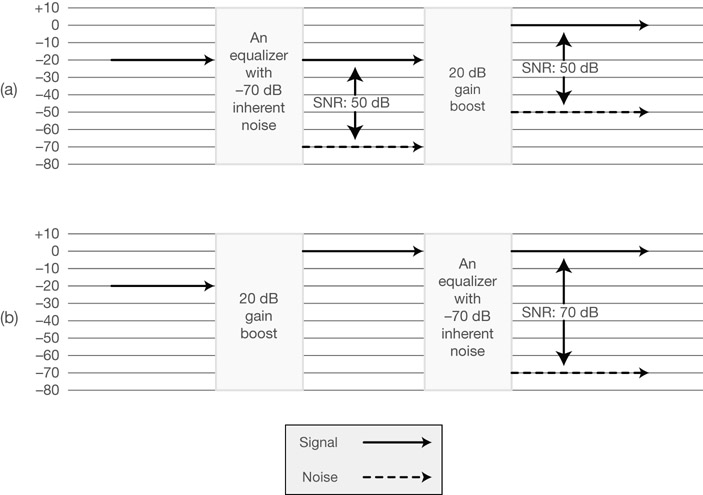
Figure 10.31 A demonstration of gain application and its effect on SNR. (a) The gain is applied after the noise is added, resulting in output signal with 50 dB SNR and noise at –50 dB. (b) The gain is applied before the noise is added, resulting in higher SNR and lower noise floor. The noise level of both the original signal and the gain stage are omitted from this illustration to keep it simple. We can assume that these are too low to be displayed on the given scale.
Correct gain structure is a tactic that helps us to reduce unwanted noise, thus improving the overall signal-to-noise ratio of our mix. Analog components are noisy—microphones, preamps, compressors, equalizers, pan pots, and analog tapes are just a few examples of components that add their inherent noise to the signal. It would be fair to say that from the point where an acoustic performance is converted into an electrical signal to the point where the same signal flows on the mix bus as part of the final mix, hundreds of analog components have added their noise. High-quality gear (such as large-format consoles) is built to low-noise specifications, but some vintage gear and cheap equipment can add an alarming amount of noise. Whatever quality of equipment is involved, simple rules can help us to minimize added noise.
The principle of correct gain structure is simple: never boost noise. Say, for example, that an equalizer has inherent noise at –70 dB, and we feed into it a signal with peak at –20 dB. The resultant output SNR (signal-to-noise ratio) will be 50 dB. If we then boost the equalizer output by 20 dB, we boost both the noise and the signal, ending up with the signal level at 0 dB but noise at –50 dB. The SNR is still 50 dB (Figure 10.31a). Now let us consider what happens if we boost the signal before the equalizer. The peak signal of –20 dB will become 0 dB as before, but the noise added by the equalizer would still be –70 dB. The output SNR will be 70 dB (Figure 10.31b).
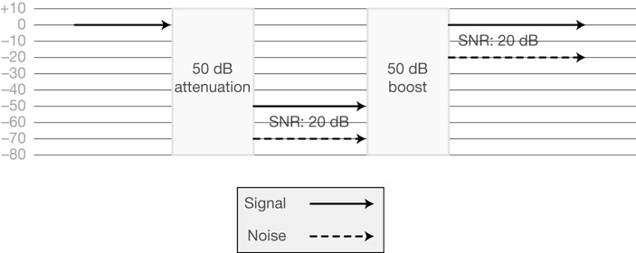
Figure 10.32 The penalty in SNR when boosting after attenuating. An incoming signal will leave the system at the same level, but the noise from the first gain stage will be boosted by the second gain stage, resulting in an output noise level of –20 dB and an SNR of 20 dB.
So when boosting the level of something, we also boost the noise of any preceding components. We can do a lot worse than attenuating something and then boosting it again. Figure 10.32 illustrates a signal at 0 dB going through two gain stages; one attenuates by 50 dB, the other boosts by 50 dB. Both stages add noise at –70 dB. The second stage will boost the noise of the first one. The input signal will leave this system with its level unaltered but with 50 dB extra noise.
To protect the signal from unnecessary boosts, the law of correct gain structure states:
Set the signal to optimum level as early as possible in the signal chain, and keep it there.
To keep the signal at optimum level, we ideally want all the components it passes through to neither boost nor attenuate it; in other words, they should all be set to unity gain. Let us look at some practical examples:
- If the channel signal is too low, is it better to boost it using the input-gain control or the channel fader?
- If the input to a reverb unit is too low, should the master aux send boost it or the input gain on the reverb unit?
- If the overall mix level is too low, should we bring the channel faders up or the mix level?
The answers to all these questions are the first option in each case, these being the earlier stage in the signal chain. If we take the first question, for example, boosting the signal using the channel fader will also boost the noise added by the compressors and equalizers preceding it. Setting the optimum level at the input-gain stage means that the compressor, the equalizer, and the fader are fed with a signal at optimum level. If the channel fader is then used to attenuate the signal, it will also attenuate any noise that was added before it. If correct gain structure is exercised, the input gain of a reverb unit should be set to unity gain (0 dB), and the level to the reverb unit should be set from the master aux send.
Correct gain structure does not mean that signals should not be boosted or attenuated— it simply helps us to decide which control to use when there is more than one option. There are, of course, many cases where boosting or attenuating is the appropriate thing to do. For example, the makeup gain on a compressor, which essentially brings back the signal to optimum level after the level loss caused by the compression process.
The digital console
Digital consoles might resemble the look of their analog counterparts, but they work in a completely different way. Analog signals are converted to digital as they enter the desk and are converted back to analog before leaving it. A computer—either a normal PC or purpose-built—handles all the audio in the digital domain, including processing and routing. The individual controls on the console surface are not part of any physical signal path— they only interact with the internal computer, reporting their state. The computer might instruct the controls to update their state when required (e.g., when a mix is recalled or when automation is enabled). Essentially, a digital desk is a marriage between a control surface and a computer.
The various controls can be assigned to many different facilities; for example, a rotary pot can control the signal level, pan position, aux send level, or equalizer gain, or even switch a compressor in and out. Most manufacturers build their consoles with relatively few controls and let the user assign them to different facilities at will. In addition, the user can select the channel to which various global controls are assigned. So, instead of having a set of EQ controls per channel strip, there will be only one global set, which affects the currently selected channel (Figure 10.33). While faders are motorized and buttons have an on/off indicator, pots are normally endless rotary controls and their position is displayed on a screen—from a small dot-display to a large, color touchscreen. The screen also provides an interface for additional functions such as metering, scene store and recall, effect library management, and various configurations.
In this realm of assignable controls, each strip can control any channel. Essentially, one strip would suffice to control all the channels a desk offers, but this would be less convenient. Manufacturers provide a set of channel strips that control threefold, fourfold, or other multiples of channels. For example, a desk with 16-channel strips might have 64 channels divided into four chunks (often called layers or banks). The user can select which layer is controlled by the channel strips at any given time (Figure 10.34). Effectively, all modern digital consoles are split consoles where many strips are organized in a few layers. The strips can also be assigned to control master aux sends and group buses. (There is, however, a dedicated fader for the mix bus.) Just like software mixers, the differences between a channel, an auxiliary bus, and a group bus are blurred. With very few exceptions, the facilities available per channel are also available for the auxiliaries and groups—we can, for example, process a group with the same EQ or compressor available for a channel.
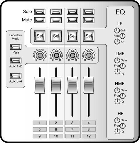
Figure 10.33 The layout of an imaginary mini-digital desk. Each strip has a single encoder, whose function is determined by the mode selection on the left. There is only one global set of EQ controls, which affects the currently selected channel.

Figure 10.34 Layers on a digital desk. The 64 channels of this desk are subdivided into four layers, each represent 16 different channels. The layer selection determines which layer is displayed on the control surface.
Assignable controls enable digital consoles to be substantially smaller than analog consoles but provide the same facilities. However, their operation is far less straightforward than the what-you-see-is-what-you-get analog concept. Thus, not all digital consoles are indeed smaller. Leading manufacturers such as NEVE intentionally build consoles as big and with as many controls as their analog equivalents in order to provide the feel and speed of an analog experience. Still, these consoles provide the digital advantage of letting users assign different controls to different facilities. Users can also configure each session to have a specific number of channels, auxiliaries, or groups. The configuration of these large desks—which might involve quite some work—can be done at home, on a laptop, and then loaded onto the desk.
For the mixing engineer, digital desks aim to provide a complete mixing solution. Dynamic range processors and multiband equalizers are available per channel, very much like on large-format consoles. Most digital desks also offer built-in effect engines, reducing the need for external effects units (although these can be connected when needed in the standard way via aux sends). They let us store and recall our mixes (often called scenes) along with other configurations. A great advantage of digital consoles is that their automation engine allows us to automate virtually every aspect of the mix—from faders to the threshold of a gate. Perhaps the biggest design difference between digital and analog consoles has to do with insert points. Breaking the digital signal path, converting the insert send signal to analog, the insert return back to digital, and making sure everything is in sync requires far more complex design and often more converters. Many desks offer insert points that, instead of being located on the digital signal path, are placed before the A/D conversion. It is still possible to use external processors that way during mixdown but in a slightly different way from on an analog desk.
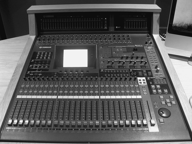
Figure 10.35 The Yamaha O2R96 studio at SAE, London. This desk provides four layers, each consisting of 24 channels (or buses). Had this desk’s layers been unfolded, it would be four times the size.