Balanced frequency spectrum

This is an ever-so-important aspect of a mix. It was suggested in Chapter 7 that, despite a vague definition of what tonal balance is, a deformed frequency response is unlikely to go unnoticed. Overemphasized or lacking frequency ranges, whether wide or narrow, is one of the critical faults that equalizers are employed to correct. They also help us to narrow or widen the frequency “size” of instruments, or shift them lower or higher on the frequency spectrum.

Shaping the presentation and timbre of instruments

Equalizers give us comprehensive control over the tonal presentation of instruments and their timbre. We can make instruments appear thin or fat, big or small, clean or dirty, elegant or rude, sharp or rounded, and so forth. A great example of this is when mixing kicks— equalizers can change their timbre in the most radical ways. Whether kicks or any other instrument, shaping the timbre and tonal presentation of instruments is one of the more creative aspects of mixing.

Separation

The frequency ranges of various mix elements nearly always overlap, a sub-bass (low-frequency sine wave) being a rare exception. Most instruments end up in a masking war that can, in some mixes at least, get quite bloody. When two or more instruments are fighting for the same frequency range, we can find it hard to discern one instrument from the other, as well as fail to perceive important timbre components or certain notes. As long as instruments are mixed together, they inevitably mask one another; we can ease the conflict by cutting from instruments any dispensable or otherwise less-essential frequencies, or in some cases by boosting important frequencies.

It is important to mention here that we do not limit each instrument to a unique frequency range—such a practice would make each instrument and the overall mix sound horrific. We combat masking until we can separate one instrument from another, and all instruments are defined to our satisfaction. Depending on the nature and density of the arrangement, this may or may not involve serious equalization.

Definition

Definition is a subset of separation. No separation equals low definition. But we also associate definition with how recognizable instruments are (provided we want them recognizable) or how natural they sound (provided we want them to sound natural). For example, in a vocal and piano arrangement there might be great separation between the two; but if the piano sounds as if it is coming from the bottom of the ocean, it is fair to say that it is poorly defined. The same can be said for a bass guitar if the notes being played cannot be discerned.

Conveying feelings and mood

Our brain associates different frequencies with different emotions. Bright sounds tend to convey a livelier, happy message, while dark sounds might be associated with mystery or sadness. Because the human voice deepens with adulthood, some believe that low-frequency attenuation of the voice gives a more youthful impression. Equalizers can be used to make vocals sweeter, a snare more aggressive, a trumpet mellower, a viola softer, etc.

Creative use

Equalizers are not employed solely for practical reasons. Creative use entails less natural or “correct” equalization that can put instruments in the limelight, give a retro feel, or create many fascinating effects.

Interest

Automating EQs is one way to add some interest to a mix. A momentary telephone effect on vocals, the rolling off of lows during a drop, and the brightening of the snare during the verse are just a few examples.

Depth enhancements

Low frequencies bend around obstacles and are not readily absorbed. High frequencies do the opposite. These are some of the reasons why we hear more low-frequency leakage coming from within venues. Our brain decodes dull sounds as if coming from farther away, which is why our perception of depth is stretched when underwater. We use this darker-equals-farther phenomenon to enhance, if not to perfect, the front/back localization of instruments in the mix.

More realistic effects

Based on the fact that high frequencies are more readily absorbed, reverbs in real rooms contain less high frequencies over time. The frequency content of a reverb also hints at the materials in rooms. Basic equalizers are often built into reverb emulators, or we can apply them externally. We will see later that filters can also reduce the size impression of a reverb.

Stereo enhancements

Frequency differences between the sound arriving at our left and right ears are used by our brain for imaging and localization. Having similar content on the left and right channels, but equalizing each differently, widens the perceived image, often creating the impression of a fuller and bigger sound. As already mentioned in Chapter 14, pan pots only utilize level differences between left and right. Stereo equalization can reinforce the pan pot function to enhance left/right localization (Figure 15.1).

Fine level adjustments

Faders boost or attenuate the full frequency spectrum of sounds. Doing so with some instruments (e.g., bass) can alter the overall frequency balance in a mix in a noticeable way. Equalizers let us modify only parts of the spectrum, therefore allowing us finer control over perceived loudness. Many instruments can be made louder by boosting around 3 kHz—our ears’ most sensitive area. The advantage in doing this is that other parts of the spectrum remain unchanged, and so masking interaction with other instruments changes less. The disadvantage, however, is that, unlike faders, EQs can negatively change the timbre of the treated instrument.

Figure 15.1 Stereo equalization (the McDSP FilterBank P6). A rather unique feature of the FilterBank range is the dual-mono mode (engaged on the left) for stereo inputs. Note that each control has a pair of sliders, each for a different channel. Only band 3 is enabled, and the different settings for each channel are evident in the two curves on the frequency-response display. Such a dual-mono feature enables stereo widening, and more realistic localization.

Better control over dynamic processors

Dynamic range processors are more responsive to low frequencies than high ones. (The reasons for this are explained later in Chapter 17, when we deal with compressors.) Because of this, the lower notes of a bass instrument might be compressed more than the high ones, resulting in inconsistent levels. Or, a kick bleed on a snare track could cause false triggering on a gate. These are just two examples of many problems that an equalizer can rectify when hooked to a dynamic range processor—a combination that also facilitates some advanced mixing techniques. This is expounded upon in the following chapters.

Removing unwanted content

Rumble, hiss, ground loops, mains hum, air conditioning, the buzz of a light dimmer, and many other extraneous noises can be imprinted on a recording. Spill is also a type of sometimes unwanted content, which gates cannot always remove. For example, gating is rarely an option when we want to remove the snare bleed from underneath the ride. Equalizers let us filter these types of unwanted sounds.

Compensating for a bad recording

The recording industry would probably have survived had a mysterious virus struck all equalizers and knocked them out for a decade or so—we would simply have had to spend more time miking and use better instruments in better studios. In the meantime, not all recordings are immaculate, so we are happy that our equalizers are healthy.

Spectral content

A sine wave is a simple waveform that involves a single frequency. Waveforms such as a square wave or a sawtooth generate a set of frequencies—the lowest frequency is called the fundamental, and all other frequencies are called harmonics. The fundamental and harmonics have a mathematically defined relationship in both level and frequencies. Figure 15.2 shows the spectral content of a 100 Hz sawtooth.

Waveforms such as sines, square waves, and sawtooths constitute the core building blocks of synthesizers. However, the natural sounds we record have far more complex spectral content, which involves more than just a fundamental and its harmonics. The spectral content of all instruments consists of four components (or partials). Combined together, these four partials constitute half of an instrument’s timbre (the other half is the dynamic envelope). These are:

• Fundamental—the lowest frequency in a sound. The fundamental defines the pitch of the sound.
• Harmonics—frequencies that are an integer multiple of the fundamental. For example, for a fundamental of 100 Hz, the harmonics would be 200, 300, 500, 500 Hz, and so forth. Harmonics are an extremely influential part of sounds—we say the fundamental gives sound its pitch, harmonics give the color.
• Overtones—frequencies that are not necessarily an integer multiple of the fundamental. A frequency of 150 Hz, for example, would be an overtone of a 100 Hz fundamental. Instruments such as snares tend to have a very vague pitch but produce lots of noise— a typical sound caused by dominant overtones.
• Formants—frequencies caused by physical resonances that do not alter in relation to the pitch being produced. Formants are major contributors to a sonic stamp—for example, our ability to recognize each person’s voice.

The spectral content of each instrument ranges from the fundamental frequency up to and beyond 20 kHz (even a kick has some energy above 10 kHz). It is worth mentioning that there might be some content below the fundamental due to body resonance or subharmonics caused by the nonlinearity of recording devices. One remarkable faculty of our brain is its ability to reconstruct missing fundamentals—whenever the fundamental or the low-order harmonics are removed, our brain uses the remaining harmonics to deduce what is missing. This is the very reason why we still recognize the lower E on a bass guitar as the lowest note, even if our speakers do not produce its fundamental frequency of 41 Hz. This phenomenon has a very useful effect in mixing and will be discussed in greater detail soon.

Figure 15.2 The harmonic content of a 100 Hz sawtooth.

Bands and associations

We already know from Chapter 7 that the audible frequency spectrum is divided into four main bands: lows, low-mids, high-mids, and highs. For convenience, the illustration shown in Chapter 7 is reproduced in Figure 15.3. The frequency spectrum can also be subdivided into smaller ranges, each with its own general characteristics. The list below provides very rough guidelines for these different ranges. All the frequencies are approximate and expressed in Hz:

• Subsonic (up to 20)—the only instruments that can produce any content in this range are huge pipe organs found in a few churches across the world. This range is felt and not heard. Although used in cinemas for explosions and thunder, it is absent from music masters.
  

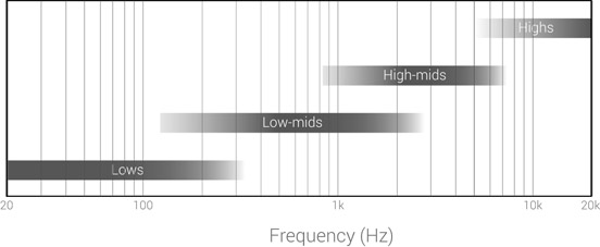
  Figure 15.3 The basic four-band division of the audible frequency spectrum.

• Low bass (20–60)—also known as “very lows,” this range is felt more than heard and is associated with power rather than pitch. The kick and bass usually have their fundamental in this range, which is also used to add sub-bass to a kick. A piano also produces some frequencies in this range.
• Mid bass (60–120)—within this range, we start to perceive tonality. Also associated with power, mostly that of the bass and kick.
• Upper bass (120–250)—most instruments have their fundamentals within this range. This is where we can alter the natural tone of instruments.
• Low-mids (250–2,000)—mostly contain the very important low-order harmonics of various instruments, thus their meat, color, and a big part of their timbre.
• High-mids (2,000–6,000)—our ears are very sensitive to this range (as per the equal-loudness curves), which contains complex harmonics. Linked to loudness, definition, presence, and speech intelligibility.
• Highs (6,000–20,000)—contain little energy for most instruments, but an important range all the same. Associated with brilliance, sparkle, and air.

The terms in the list above are just a few of many we associate with the various frequency ranges. We also have terms to describe deficiency and excess of various ranges. We use these terms in verbal communication, but we might also use them in our heads—first, we decide that we want to add spark and then we translate it to a specific frequency range. These terms are not standardized, and different people might have different ideas about particular terms. One thing is certain—the frequency ranges we associate these terms with are very rough. The body of a bass guitar is very different from the body of a flute. Figure 15.4 lists these terms.

Sibilance

Sibilance is the whistling sound of s, sh, ch, and sometimes t. “Locks in the castle” has two potentially sibilant consonants. Languages such as German and Spanish have more sibilant constants than English. The same sentence in German—”schlösser im schloss”— has four potentially sibilant consonants. Sibilance is normally found between 2 and 10 kHz and can be emphasized by certain microphones, tube equipment, or just standard mixing tools such as equalizers and compressors. Emphasized sibilance pierces through the mix in an unpleasant and noticeable way. It would also distort on radio transmission and when cut to vinyl.

It is important to note that not all speakers produce the same degree of sibilance. One must be familiar with one’s monitors to know when sibilance has to be treated and to what extent. Mastering engineers would probably agree that too many mixes require sibilance treatment. So, if in doubt when mixing, better safe than sorry.

Filters, equalizers, and bands

Faders attenuate or boost the whole signal. Put another way, the whole frequency spectrum is made softer or louder. Equalizers attenuate or boost only a specific range of frequencies, and by that they alter the tone of the signal. Early equalizers could only attenuate (filter) frequencies; later designs could boost as well. Regardless, all equalizers are based on a concept known as filtering; thus, the terms “equalizer” and “filter” are used interchangeably. In this text, we will use the term filter to mean a circuit that acts with reference to a single frequency, and equalizer for a device that might consist of a few filters.

A filter might be in charge of a specific range of frequencies known as band. A typical equalizer on a large-format console has four bands: LF, LMF, HMF, and HF (low fre quencies, low-mid frequencies, high-mid frequencies, and high frequencies). There would normally also be a high-pass filter (HPF) and a low-pass filter (LPF). Such an equalizer is shown in Figure 15.5. Many software plugins and digital equalizers provide more than four bands, with some plugins offering 10 or more. Such equalizers are known as paragraphic EQs, and are a hybrid between parametric and graphic equalizers (both explained soon). In many cases, a graph on the plugin window shows the combined frequency response of all bands. A paragraphic EQ plugin is shown in Figure 15.6.

This is probably the right time to look at the difference between the two types of equalizers shown in Figures 15.5 and 15.6. It can be argued that we rarely need more than what is offered by the analog equalizer shown in Figure 15.5—it provides two pass filters to remove content, two shelving filters to change the general tonality of sounds, and two parametric equalizers for more focused treatment. Essentially, most productions before the DAW age were mixed with equalizers that were no more lavish than the one above. Software plugins with a multitude of bands, say 10, can fool people into thinking that standard equalization requires that many bands. It is true that sometimes many bands are useful, but this is more often the case with problematic recordings. For general tone shaping, it is often seasoned engineers that have sufficient auditory skill to take advantage of such a magnitude of bands. Equalization is not the easiest aspect of mixing, and introducing more bands can make it harder. It is better to hit the right spot with one band than miss it with three.

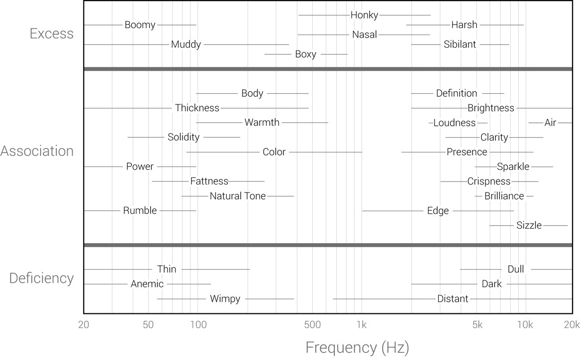
Figure 15.4 Subjective terms we associate various frequency ranges with, and excess or deficiencies in these ranges. The terms are not standardized, and the frequency ranges are rough.

Figure 15.5 A diagram of the SSL 4000 G+ equalizer. The equalizer section consists of four bands: the LF and HF bands are shelving filters; the LMF and HMF are parametric equalizers. At the top are high- and low-pass filters.

Another potential problem with paragraphic plugins is the response plot they present. These can easily divert the attention from the actual sonic effect of equalization and lead people to equalize by sight alone. For example, one might over-boost on an equalizer simply because a 6 dB boost on its frequency plot looks graphically small. If you have ever boosted on a paragraphic plugin then looked at the gain value to see why the effect is so extreme or little, you’ve probably been equalizing by sight. Professional engineers working on analog desks hardly ever use their eyes while equalizing—you will notice that the gain scales in Figure 15.5 are not even labeled. McDSP lets the user choose whether or not to view the response plot, promoting hearing-based equalization for those who fancy it. It might be wise for other manufacturers to follow suit.

Figure 15.6 A paragraphic equalizer plugin (Digidesign’s DigiRack 7-band EQ 3). This plugin provides seven bands. Two are high and low filters, and the other five are parametric filters, although the LF and HF bands can be switched into shelving mode.

Frequency-response graphs

We use frequency-response graphs to demonstrate how a device alters the different frequencies of the signal passing through it (Figure 15.7). On these gain vs. frequency graphs, the frequency axis covers the audible frequency range between 20 Hz and 20 kHz. The fact that our perception of pitch is not linear is evident on the frequency scale: 100–200 Hz has the same width as 1–2 kHz. The spacing between the grid lines corresponds to their range (10 Hz steps for tens of hertz, 100 Hz for hundreds of hertz, and so forth).

The filter in Figure 15.7 is known as a brick-wall filter. It has a step-like response that divides the frequency spectrum into two distinct bands, where all frequencies to one side are removed and all frequencies to the other are retained. A filter with such a vertical slope is hypothetical—it cannot be built, and even if it could be it would bring about many unwanted side effects. Yet the term brick-wall filter is sometimes used to describe a digital filter with a very steep slope, although never vertical.

There are so many terms and circuit designs involved in filters that it can be very hard to keep track of them all. To generalize, in mixing we use the following types: pass, shelving, and parametric. Each type has a recognizable shape when shown on a frequency-response graph. Regardless of the filter we use, there is always a single reference frequency (e.g., 800 Hz in Figure 15.7), and in most cases we have control over it. This frequency has a different name for each type of filter.

Figure 15.7 A brick-wall filter on a frequency-response graph. The filter in this graph removes all frequencies below 800 Hz, but lets through all the frequencies above. This type of brick-wall filter only exists in theory.

Pass filters

The circuitry of a pass filter can be as simple as a mere combination between a capacitor and a resistor. The reference frequency of pass filters is called the cut-off frequency. Pass filters allow frequencies to one side of the cut-off frequency to pass, while continuously attenuating frequencies to the other side. A high-pass filter (HPF) allows frequencies higher than the cut-off frequency to pass, but filters frequencies below it. A low-pass filter (LPF) does the opposite—it lets what is below the cut-off frequency through, while filtering what is above it. Figure 15.8 illustrates this.

It is easy to notice that the cut-off points in Figure 15.8 are not where the curve starts to bend (the transition frequency). Indeed, the cut-off frequency on pass filters is where 3 dB of attenuation occurs. For example, it is 100 Hz for the HPF in Figure 15.8. As a consequence, we can see that a short range of frequencies has been affected despite being higher than the cut-off frequency (or lower, in the case of LPF).

Figure 15.8 A high-pass and a low-pass filter.

Some filters have a fixed cut-off frequency and only provide an in/out switch. In many cases, the fixed frequency of an HPF would be around 80 Hz, which is right below the lowest note of a regular guitar (E, 82 Hz) and the second harmonic of the lowest note on a bass guitar (E, 41 Hz). However, the majority of the pass filters we use in mixing let us sweep the cut-off frequency.

Another characteristic of a pass filter is slope. This determines the steepness of the filter curve. The slope is expressed in dB per octave (dB/oct or dB/8ve), with common values being a multiple of six. A gentle slope of 6 dB/oct means that below the cut-off frequency, each consecutive octave experiences an additional 6 dB of gain loss. With an aggressive slope of 30 dB/oct, it will only take two octaves before frequencies are attenuated by more than 60 dB (a point that can be perceived as effective muting). Generally, the steeper the slope, the more unwanted effects the filter produces. Figure 15.9 shows different slopes. The 6 dB multipliers are set in stone in analog EQs, and rarely can we alter the slope of a filter. An analog pass filter often has a fixed slope of either 6, 12, or 18 dB/oct (in order of popularity). A slope of 36 dB/oct is considered very steep. It is easier in digital designs to offer a variety of slopes, and they are not always bound to 6 dB/oct steps. It should be mentioned that if we do not have slope control, we could achieve our desired slope by combining two filters. For example, we can achieve a 12 dB/oct response by combining two 6 dB/oct filters with the same cut-off frequency. As the signal travels through the first filter, the first octave experiences maximum attenuation of 6 dB; as it travels through the second filter, the same octave experiences an additional 6 dB of attenuation, resulting in a summed response of 12 dB/oct. In the analog domain, this involves connecting two pass filters in a series. With a paragraphic plugin, this involves having two bands set to the same pass response. In all cases, the cut-off frequencies of the two filters should be identical.

Figure 15.9 Different slopes on an HPF. These four instances of the Digidesign DigiRack EQ 3 illustrate a different slope each. From top to bottom: 6, 12, 18, and 24 dB/oct. The cut-off frequency is set to 1 kHz and is clearly indicated with a white circle.

Figure 15.10 Pass filter resonance (the PSP MasterQ plugin). The Q control on the HPF section acts as a resonance control. The resonance is seen as a bump around the cut-off frequency.

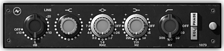
Figure 15.11 The Universal Audio NEVE 1073 EQ plugin. This plugin, which emulates the sound of the legendary analog NEVE 1073, has a frequency response that deviates from the perfect theoretical shape of filters, a fact that contributes to its appealing sound. The high-pass filter (rightmost control) involves changing the resonance for each of the four selectable cut-off frequencies.

Many of us are familiar with the pass filters on synthesizers that have both cut-off and resonance control. Resonance provides a boost around the cut-off frequency, and gives some added edge to the transition range. Resonance is highly noticeable when the cutoff frequency is swept, and most DJ mixers incorporate resonant filters. Resonance is not an extremely common feature in mixing equalizers, although some, such as the PSP MasterQ in Figure 15.10, do provide it. However, it might still be “secretly” incorporated into some designs, often those that offer very few controls and do not reveal their frequency-response graph (typically analog or the digital plugins that emulate them). One such example is the Universal Audio NEVE 1073 EQ, shown in Figure 15.11. Generally speaking, equalizers of this kind have a frequency response that is far from textbook perfect (such as Figure 15.8), a fact that often contributes to their appealing sound. Even if an equalizer does not offer a resonance control, we can achieve this characteristic by adding a parametric filter around the cut-off frequency. Figure 15.12 illustrates how this is done. The only limitation with such a setup is that both reference frequencies have to be adjusted if we want to sweep the resultant response.

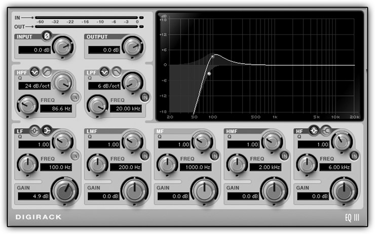
Figure 15.12 Combining two bands to create a resonant filter (the Digidesign DigiRack 7-band EQ 3). A parametric filter (LF band) is used to create a bump around the cut-off frequency of an HPF, resulting in a response typical of a resonant filter.

Shelving filters

Most people have used shelving filters—these are the bass and treble controls found in our domestic hi-fi systems, also known as tone controls. Shelving filters, as they are now known, were conceived by Peter Baxandall in the late 1940s. They are so-called as their response curve can, in inspiring moments at least, remind us of shelves.

Unlike pass filters, which only cut frequencies, shelving filters can also boost. The reference frequency of shelving filters divides the spectrum into two bands. On one side, frequencies are undisturbed; on the other, frequencies are either attenuated or boosted by a constant amount. A gain control determines that amount. As per the above discussion about vertical response slopes being impossible, there is always a transition band between the unaffected frequencies and those affected by the set gain. Figure 15.13 shows the four possible versions of shelving filters.

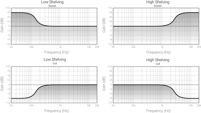
Figure 15.13 The four versions of shelving filters. For boost, +9 dB of gain is applied; for attenuation, –9 dB.

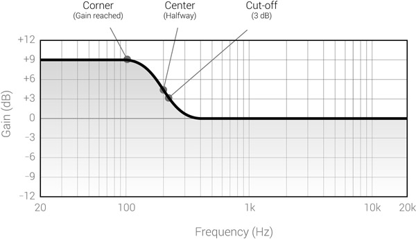
Figure 15.14 Three possible options for the shelving frequency. The corner frequency is where the set gain is reached. The center frequency is halfway through the transition band. The cut-off frequency is the traditional 3 dB point.

When it comes to defining what is the reference frequency of shelving filters, we encounter ambiguity. Designers might choose one of the three main possibilities (illustrated in Figure 15.14). Some define it in the traditional engineering sense as the point at which 3 dB of gain is reached—the familiar cut-off frequency. However, this tells us little about the real effect of the filter, which roughly happens when the set amount of gain is reached. Since this is often what we are after, some designers use this point as a reference, and it is called the corner frequency. To add to the confusion, it is also possible for the reference frequency to be halfway on the transition range—a frequency we can regard as the center frequency. Of all three options, it can be argued that the corner frequency is the most intuitive one to work with.

All shelving filters offer control over the gain amount, often ranging between –12 and +12 dB. Most filters in mixing also offer control over the shelving frequency. Some filters also offer slope control, which determines the steepness of the slope in the transition band. Just like with pass filters, the actual response of shelving filters might deviate from the curves shown in Figure 15.13. In fact, it is likely to deviate. One very common response involves a contrast resonance around the transition frequency; that is, a section of the curve that bends in the opposite direction to the normal response. Such a response can be seen in Figure 15.15.

Figure 15.15 A typical contrast resonance on a shelving filter (the Universal Audio Cambridge EQ). Both the low- and high-shelving filters are engaged in this screenshot, and it might be easier to discern them if we imagine a cross-line at 700 Hz. The low-shelving filter, set to type A, has a single contrast bend around the transition frequency. The high-shelving filter, set to type C, has two of these bends—one around the transition frequency, the other around the corner frequency.

Parametric filters

In 1972 at the AES, George Massenburg unveiled the parametric equalizer—a revolutionary circuit that he designed with help from fellow engineers. Although the concept of bandpass and band-reject filters (primitive types of parametric filters) was already well established, parametric equalizers became, and still are, de facto in mixing.

Figure 15.16 A parametric filter. Both response graphs involve 9 dB of gain (boost or cut) and a center frequency at 400 Hz; 3 dB below the center frequency are the two cut-off frequencies at 200 and 800 Hz. The two-octave bandwidth (200–800 Hz) is measured between the two cut-off points.

Parametric filters can cut or boost. Their response curve is reminiscent of the shape of a bell, as can be seen in Figure 15.16. The reference frequency is called the center frequencyand we can sweep it higher or lower. The gain determines the maximum amount of boost or cut reached at the center frequency. The two cut-off points are 3 dB away from the center frequency (3 dB below for boost, 3 dB above for cut). The bandwidth is measured between these two cut-off points, and we express it in octaves.

Had we expressed the bandwidth in hertz (for example, 600 Hz for the graphs in Figure 15.16), the effect of the filter would alter as the center frequency is swept, where the higher the frequency is, the less the effect. Consequently, the bell shape would narrow as the center frequency is swept higher. The reason for this has to do with our nonlinear pitch perception. To demonstrate this again, 600 Hz between 200 and 800 Hz equals two octaves (24 semitones); the same 600 Hz between 10,000 and 10,600 Hz is only a semitone. There is no comparison between affecting two octaves and a semitone.

Although the bandwidth on some equalizers is expressed in octaves, it is far more common to use a parameter called Q (quality factor). Q can be calculated by the mathe matical expression Fc/ (Fh – Fl), where Fc is the center frequency and Fh and Fl represent the high and low cut-off frequencies, respectively. The higher the Q, the narrower the shape of the bell. Roughly speaking, Q values range from 0.1 (very wide) to 16 (very narrow). Three different Q settings can be seen in Figure 15.17.

Figure 15.17 Different Q settings (the Cubase StudioEQ). Three bands are engaged in this screenshot, all with a gain boost of 15 dB. The lowest band (leftmost) shows a response with a narrow Q (10). The middle band response is achieved with a moderate Q (2.5). The widest Q (0.5) is applied on the highest band. The different bandwidths can be visualized by looking at the +12 dB grid line between the cut-off points.

The shape of the bell gives the filter much of its characteristics, and it is not surprising that many variants exist. One important aspect is whether or not there is a dependency between the gain and the Q (Figure 15.18). With some designs, the bell narrows with gain (a behavior described as proportional Q). As a consequence, changing the gain might also require adjustment to the Q. Equalizers of this type tend to sound more forceful as they become sharper with higher gain settings. A design known as constant Q provides an alternative where the bandwidth is (nearly) constant for all gain settings. This produces a softer effect that often brings about more musical results.

Figure 15.18 Proportional vs. constant Q. With proportional Q, the bandwidth varies in relation to the gain; with constant Q, it remains the same.

Most of the sounds we are mixing have a rich and complex frequency content that mostly ranges from the fundamental frequency to 20 kHz and beyond. The timbre components of various instruments do not exist on a single frequency only, but stretch across a range of frequencies. One of the accepted ideas in equalization is that sounds that focus on a very narrow frequency range are often gremlins that we would like to remove. To accommodate this, designs provide an attribute called boost/cut asymmetry, which has grown in popularity in recent years. In essence, an asymmetrical filter of this type will use wider bell response for boosts, but a narrower one for cuts. We, the users, see no change in the Q value. This type of asymmetrical response is illustrated in Figure 15.19.

A variation of parametric filter is known as a notch filter. We use this term to describe a very narrow cut response, such as the cut in Figure 15.19. This type of response is often used to remove unwanted frequencies, such as mains hum or strong resonance.

Figure 15.19 Cut/boost asymmetry (the Sonnox Oxford Equalizer and Filters plugin). Both the LMF and HMF are set with extreme gain of –20 and +20 dB, respectively. The Q on both bands is identical (2.83). The asymmetry is evident as the cut response is far narrower than the boost response. This characteristic is attributed to the EQ-style selection seen as Type-2 in the center below the plot. Other EQ styles on this equalizer are symmetrical.

A summary of pass, shelving, and parametric filters

It is worthwhile at this stage to summarize the various filters we have looked at so far. The McDSP plugin in Figure 15.20 will help us recap.

A pass filter continuously removes frequencies to one side of the cut-off frequency. Normally we have control over the cut-off frequency, and occasionally we can also control the slope. The HPF and LPF are bands 1 and 6, respectively, in Figure 15.20.

Figure 15.20 The McDSP FilterBank E6.

A shelving filter boosts or attenuates frequencies to one side of the corner frequency. Normally we can control the corner frequency (or any other reference frequency if different) and gain. The shelving bands in Figure 15.20 are 2 and 5. The FilterBank E6 also provides control over the peak and dip resonance and the slope.

A parametric filter normally provides gain, frequency, and Q. The set gain is reached at the center frequency, and the Q (or octave bandwidth) determines the width of the bell between the two cut-off points. Bands 3 and 4 in Figure 15.20 are parametric filters. A parametric filter that offers variable gain, frequency, and Q is known as a (fully) parametric equalizer. A parametric filter that only offers variable gain and frequency is known as a semi-parametric or sweep EQ.

The response characteristics of various filter designs give each equalizer its unique sound. Deviations from the textbook-perfect shapes, among other factors, gave many famous analog units their distinctive and beloved sounds. To our delight, it is not uncommon nowadays to come across professional plugins that provide different types of charac teristics to choose from and more control over the equalizer response.

Dynamic equalizers

Dynamic equalizers are not currently that popular and are often associated with mastering applications. Yet, the plugin revolution means that we should expect to see more of them in the future, and they can be just as beneficial in mixing as they are in mastering.

Figure 15.22 Basic diagram of single-band dynamic EQ. The frequency and Q settings determine both the equalizer settings and the pass-band frequencies that the gain computer is fed with. Basic compressor controls linked to the gain computer dictate the amount of cut or boost applied on the EQ.

Figure 15.23 Dynamic EQ plugin (the t.c. electronic Dynamic EQ). Both bands 1 and 4 are active in this screenshot. Looking at each band, the darkest area (most inward) shows static equalization, the light area shows dynamic equalization, and the gray area (most outward) shows the band-pass filter response curve.

In contrast to the standard (static) equalizer, where the amount of cut or boost on each band is constant, the same amount on a dynamic equalizer is determined by the gain intensity on each band. Put another way, the louder or softer a specific band becomes, the less or more cut or boost is applied. Dynamic equalizers are something of a marriage between a multiband equalizer and a multiband compressor. For each band, we often get the familiar compressor controls of threshold, ratio, attack, and release. Unlike multiband compressors, these do not control the gain applied on the frequency band, but the amount of boost or cut on the equalizer of that band. Figure 15.22 provides a diagram of a one-band dynamic equalizer, while Figure 15.23 shows a multiband dynamic EQ.

Dynamic equalizers are very useful when we want to correct varying frequency imbalances, such as those caused by the proximity effect. We can set the EQ to cut more lows when these increase in level. We can also reduce finger squeaks on a guitar only when these happen. There are many more fascinating applications, but these are explored in Chapter 17, which is about compressors, as they are more common at present than dynamic equalizers.

Equalization and solos

Mostly, equalization is done in mix-context. Solving masking or tuning an instrument into the frequency spectrum is done in relation to other instruments. Equalizers and solo buttons are not exactly best friends. Instruments that sound magnificent when soloed can sound awful in the mix. The opposite is also likely—an instrument that sounds dreadful when soloed can sound great in the mix. If we apply high-pass filtering to soloed vocals, we are likely to set a lower cut-off point than we would have had we listened to the whole mix— in isolation, we only hear what the filter removes from the sound, but we cannot hear how this removal can give the vocals more presence and clarity in the mix. Yet, there are several situations where we equalize while soloing. Mostly, this involves initial equalization and instances where the mix clouds the details of our equalization. But it is worth remembering that:

Upward vs. sideways

An old engineering saying is that if a project was recorded properly, with the mix in mind, there would be little or no equalization to apply. To some recording engineers, this is a major challenge. We say once sounds are recorded that they exist in their purest form and any equalization is interference with this purity. In subtle amounts, equalization is like makeup. But in radical amounts, it is like pretty drastic plastic surgery—it can bring dreadful results. I like to compare equalizers to funfair mirrors—gently curved mirrors can make you slimmer, broader, taller, or shorter, which sometimes make you look better. But the heavily curved mirrors just make you look funny and disproportionate. Having said that, as part of the sonic illusion we provide in some mixes, equalizers are used generously for extreme manipulations of sounds. The natural vs. artificial concept is very relevant when it comes to equalization.

There is no doubt that some equalizers lend themselves better to our artistic intentions than others, but they all share common issues. The more drastically we employ them, the more we stand to lose in return. In that sense, a perfect EQ is one that has a flat frequency response, and thus no effect at all. In this ideal state, we are more likely to impair the sound with:

• more gain;
• narrower Q settings;
• steeper slopes; and
• more angular transition bends.

Still, equalizers are not that injurious—they are widely used in mixes and yield magnificent results. The point is that sometimes we can achieve better results with a slight change of tactic—one that simply involves less drastic settings.

Say, for example, Sid wants to add attack to a kick. Sid reads in some book that the kick’s attack is at 6 kHz. So he dials a parametric EQ to that frequency, and the more attack he wants, the more he boosts the gain. Sid equalizes upward. He ends up with narrow Q and +12 dB of gain. Nancy knows that very few specific sounds focus on a narrow frequency range, and these are often gremlins that we want to remove, not emphasize. So she dials a frequency of 6 kHz as well, but with wider Q and lower gain. Nancy works sideways. Nancy boosts less, but boosts a wider range of the kick’s attack, so the overall impact is roughly the same, only with less artifacts. This example is illustrated in Figure 15.24a.

We can use the same example with other types of filters. We can set a high-shelving filter at one frequency with more gain or set it to a lower frequency with lower gain (Figure 15.24b). Similarly, we can set an HPF with a steep slope at one frequency or we can set a gentler slope at a higher frequency (Figure 15.24c). The performance of a pass filter is often evaluated by how well it handles the transition area, especially with steeper slopes. Cheap designs can produce very disturbing side effects around the cut-off frequency. The three examples in Figure 15.24 can be summarized as:

We must not forget that, as with many other mixing tools, sometimes we are more interested in hearing the edge—subtlety and transparency is not always what we are after. For example, in genres such as death metal, equalizers are often used in what is considered a radical way, with very generous boosts. The equalizer’s artifacts are used to produce harshness, which works well in the context of that specific music. Some equalizers have a very characteristic sound that only sharpens with more extreme settings.

Equalizers and phase

The operation of an equalizer involves some delay mechanism. The delays are extremely short, well below 1 ms. Group delay is a term often used, suggesting that only specific fre quencies are delayed—while not strictly precise, it is faithful to the fact that some frequencies are affected more than others. Regardless, the delay mechanism in equalizers results in unwanted phase interaction. Just like two identical signals that are out of phase result in comb filtering, we can simplify and say that an equalizer puts some frequencies out of phase with other frequencies, resulting in phasing artifacts. We always see the

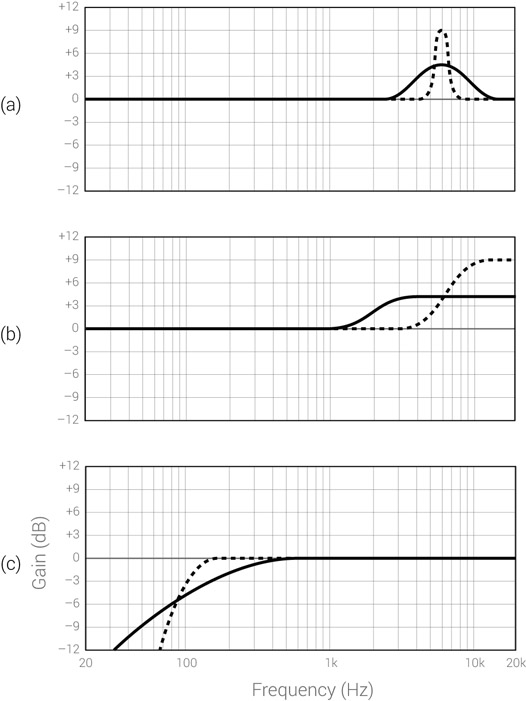
Figure 15.24 Equalization alternatives. In all these graphs, the dashed curves involve more drastic settings than the solid curves. The dashed and solid curves could bring about similar results, although the dashed curves are likely to yield more artifacts. This is demonstrated on a (a) parametric filter, (b) shelving filter, and (c) pass filter.

frequency-response graph of equalizers, but rarely see the frequency vs. phase graph, which is an inseparable part of an equalizer’s operation. Figure 15.25 shows such a graph for a parametric equalizer.

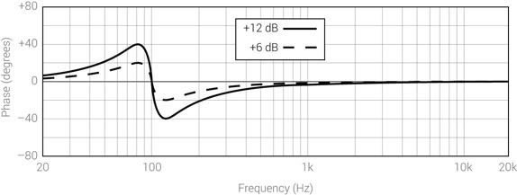
Figure 15.25 The phase response of a boost on a parametric equalizer. The equalizer center frequency is 100 Hz. The solid line shows a boost of 12 dB, and the dashed line shows a gain boost of 6 dB.

There are two important things we can learn from Figure 15.25. First, that the higher the gain is, the stronger is the phase shift. Second, we can discern that frequencies near the center frequency experience the strongest phase shifts. This behavior, although demonstrated on a parametric EQ, can be generalized for all other types of EQ—the more gain there is, the more severe phase artifacts become, with the greatest effect taking place around the set frequency.

One interesting question is: What happens with phase when we cut rather than boost? Figure 15.26 shows the same settings as in Figure 15.25, only this time for cut rather than boost. We can see that the only difference is that the two response graphs are mirrored, but the phase extent remains the same. It is a myth that equalizers cause more phase shift when we boost—there is nothing in the science of either analog or digital filters to support such a claim. However, it is correct that we notice the phase shift more when we boost, for the simple reason that we also make the phase artifacts louder. It is therefore not surprising that many mixing engineers prefer to attenuate rather than boost when equalizing, and that many sources give such a recommendation. Also, when boosting we risk clipping.

There is one type of digital equalizer that has a flat phase response—the linear phase equalizer (Figure 15.27). Digital filters are based on mathematical formulae. These formulae have stages, and the audio travels through the different stages. By making the formula of a filter symmetrical, as audio travels through one side of the formula its phase is shifted, but once it has gone through the mirrored side it shifts back in phase to its original inphase position. One issue with linear phase equalizers is that they require extensive processing power and a large buffer of audio (bigger than the typical 1,024 samples often provided by the audio sequencer). Thus, they are CPU-consuming and introduce plugin delay. Designers have to compromise between phase accuracy, processing power, and the delay the plugin introduces.

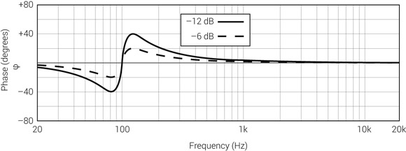
Figure 15.26 The phase response of a cut on a parametric equalizer. This is the same equalizer as in Figure 15.25, only this time with gain cut instead of boost.

While linear phase equalizers rectifies one artifact of equalization, they do not rectify them all. Like standard equalizers, linear-phase ones have many other unwanted byproducts such as ringing, or lobes and ripples.

Linear phase equalizers may sound more “expensive.” They are said to excel at retaining detail, depth, and focus. They are generally less harsh and likely to be more transparent. But many of the unwanted artifacts we encounter with standard equalizers (including those we associate with phase) are also a product of linear phase equalizers. In addition, transients might not be well handled by the linear phase process. In fact, there are situations where standard equalizers clearly produce better results. Thus, linear phase equalizers provide an alternative, not a superior replacement.

Figure 15.27 A linear phase equalizer (the PSP Neon). This plugin offers eight bands with selectable filter type per band. It is worth noting the LP (linear phase) button, which enables toggling between linear phase and standard mode.

The frequency yin-yang

Figure 15.28 shows what I call the frequency yin-yang. I challenge the reader to identify what type of filter this is. Is it a +12 dB high-shelving filter brought down by 6 dB? Or is it a –12 dB low-shelving filter brought up by 6 dB? The answer is that it can be both, and, following our discussion about phase shift not varying between cut and boost, the two options should sound identical.

Figure 15.28 The frequency yin-yang.

Regardless of which of the two ways the frequency yin-yang is achieved, it teaches us something extremely important about our frequency perception: provided that the final signal is at the same level, boosting the highs or reducing the lows has the same effect. To make something brighter, we can either boost the highs or attenuate the lows. To make something warmer, we can boost the low-mids or attenuate from the high-mids up. While this concept is easily demonstrated with shelving filters, it works with other filters all the same. For example, to brighten vocals, we often apply HPF, and, despite removing a predominant low-frequency energy, the vocals can easily stand out more. Adding both highs and lows can be achieved by attenuating the mids. Sure, in many cases we have a very specific range of frequencies we want to treat, but it is worth remembering that sometimes there is more than one route to the same destination.

One more example is necessary here. If we stop thinking about individual treatment, we can apply the frequency yin-yang at mix level as well. Say we want to add attack to a kick. Instead of boosting the attack frequency on the kick, we can attenuate the same frequency on masking instruments. In fact, a common technique based on this concept is called mirrored equalization. It involves a boost response on one instrument and mirrored response on another. This helps reduce frequency overlapping, and the same effect can be achieved with less gain on each filter. Figure 15.29 illustrates this.

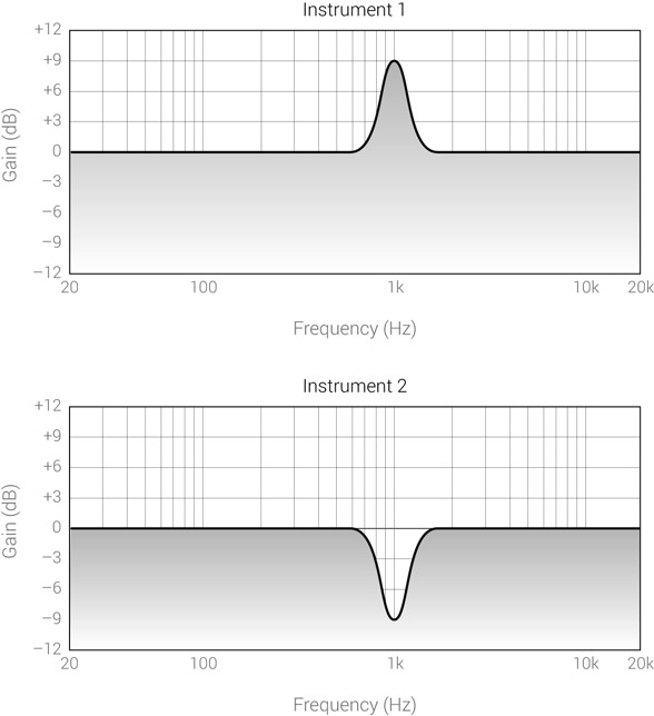
Figure 15.29 Mirrored equalization. A boost on one instrument is reinforced by mirrored response on a masking instrument.

Equalization and levels

By altering the level of a specific frequency range, we also alter the overall level of the signal. As per our axiom, louder-perceived-better, A/B comparisons can be misleading— we might think it is better when boosting on the equalizer and worse when attenuating. In order to allow fair A/B comparisons, some equalizers provide an output level control. After equalizing, we match the level of the processed signal to the unprocessed signal, so our critical judgment is purely based on tonality changes, not level changes. While it is understood why output level control is not found on the small EQ sections of even the largest consoles, it is unclear why many plugin developers overlook this important feature.

A/B comparison aside, the louder-perceived-better principle can lead to immediate misjudgments as we equalize, before compensating for the gain change. The risk is the same—we might think boosting improves the sound purely due to the overall level increase. The frequency yin-yang can minimize that risk; by taking the attenuation route, we are less likely to base our evaluation on the overall level factor. It was just mentioned that attenuating the lows of vocals could increase their presence. By attenuating a specific frequency range, we reduce masking on that specific range. Reducing the lows of the vocals, for example, would increase the low-end definition of other instruments. If by any chance the loss of overall level bothers us, we can always compensate for it. By boosting a specific frequency range, we increase masking. The equalized instrument becomes more defined, but on the specific boosted range it masks more. This is why it is recommended to consider attenuation before boosting.

The psychoacoustic effect of taking away

In the first instance, our ears tend to dislike the attenuation or removal of frequencies. By attenuating or removing, we take away something and make instruments smaller. Our brains might need some time to get used to such changes. By way of analogy, it is like having a drastic haircut—it might feel a bit weird on the first day, but we get used to it after a while. Both listening in mix-perspective and giving the equalization effect some time to settle in can be beneficial when we take away some frequency content.

One specific technique that can be used to combat this psychoacoustic effect is making an instrument intentionally smaller than appropriate, forgetting about the equalization for a while, then going back to the equalizer and making the instrument bigger. This could allow a fairer judgment when deciding how to equalize as we make things bigger rather than smaller.

Applications of the various shapes

Having the choice between pass, shelving, and parametric filters, we employ each for a specific set of applications. The most distinct difference between the various shapes puts pass and shelving against the parametric filter. Both pass and shelving filters affect the extremes of the frequency spectrum. Parametric filters affect a limited, often relatively narrow bandwidth, and rarely do we find them around the extremes. In a more specific context, the basic wisdom is this:

• Pass filters—used when we want to remove content from the extremes. For example, low-frequency rumble.
• Shelving filters—used when we want to alter the overall tonality of the signal (partly like we do on a hi-fi system), or to emphasize or soften the extremes. For example, softening exaggerated low-frequency thud.
• Parametric filters—used when what we have in mind is a specific frequency range or a specific spectral component. For example, the body of a snare.

It is sensible to introduce the three different types into a mix in this order: first use pass filters to remove unwanted content, then use shelving for general tonality alterations, and finally use parametric filters for more specific treatment. The following sections detail the usage of each filter type.

HPFs

HPFs are common in mixes of recorded music. First, they remove any low-frequency gremlins such as rumble or mains hum. Then, recorded tracks can contain a greater degree of lows than needed in most mixes (sometimes due to the proximity effect; sometimes due to the room). When the various instruments are mixed, the accumulating mass of low-end energy results in muddiness, lack of clarity, and ill definition. HPFs tidy up the low-end by removing any dispensable lows or low-mids. Doing so can clear some space for the bass and kick, but more importantly it can add clarity and definition to the treated instrument. This is worth stressing:

An HPF might be applied on every single instrument. Vocals, guitars, and cymbals are common targets. Vocals, nearly by convention, are high-passed at 80 Hz—a frequency below which no contributing vocal content exists. Higher cut-off frequencies are used to remove byproducts of the proximity effect or some body that might not have a place in the mix. Many guitars, especially acoustics, occupy unnecessary space on the lows and low-mids, which many other instruments can use instead. When acoustic guitars play a rhythmic role, they are often filtered quite liberally with most or all of their body removed. Cymbal recordings often involve some drum bleed that cannot be gated (e.g., removing the snare from underneath the ride), so the filter also acts as a spill eliminator. Pianos, keyboards, snares, and any other instrument can benefit from low-end filtering all the same. We sometimes even filter the kick and bass in order to mark their lowest frequency boundary, and in turn that of the overall mix.

The frequencies involved in this tidying up process are not strictly limited to the lows. Cymbals, for example, might be well within the low-mids. A possible approach is to simply sweep up the cut-off frequency until the timbre of the treated instrument breaks, then back it off a little. Usually, the busier the mix, the higher frequency HPFs reach. Over-filtering can create a hole in the frequency spectrum or reduce warmth. To rectify this, we can pull back the cut-off frequency on some instruments.

One interesting characteristic of HPFs is that they can be pushed quite high before we notice serious impairment to the treated instrument. The reason for this has to do with our brains’ ability to reconstruct missing fundamentals. What an HPF removes, the brain reconstructs—we clear space in the mix, but do not lose valuable information.

HPFs can manipulate the characteristics of reverbs. Generally speaking, the size, depth, and impression of a reverb all focus on the lower half of the spectrum (lows and low-mids). The highs mostly contribute some definition and spark. By filtering the lows, we can reduce the size of a reverb and its resultant depth. The higher the cut-off frequency is set, the smaller the size becomes. Although we have full control over the size and depth of a reverb when using a reverb emulator, these factors are imprinted into a reverb captured on recordings.

HPFs are also used to remove pops—low-frequency air bursts caused by Ps, Bs, or any other plosive sounds such as an emphasized “who.” The higher the cut-off frequency is, the more the pop is reduced, but also the more likely the timbre is to suffer. In the days of tapes, removing these pops required filtering the whole vocal track and compromises had to be made. Audio sequencers offer a much more elegant solution, filtering the pop only. This is achieved using offline processing, where we simply select each pop, apply filtering, then crossfade to prevent clicks. Figure 15.30 illustrates this.

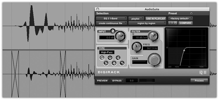
Figure 15.30 Pop removal using offline processing. The top track, before pro cessing, shows an evident pop. An offline HPF is set with a cut-off frequency of 368 Hz. Had the filter been applied in real time throughout the track, much of the vocal’s thickness would have been lost. The offline process was only applied on a limited selection that included the pop and some margins for the crossfades. The crossfades were then applied to prevent clicks. The resultant bottom track shows the apparent energy loss of the pop.

LPFs

Unlike their lofty twin, LPFs are somewhat neglected when it comes to mixing. Unfortunately, our ears do not reconstruct the higher harmonics once lost, so we find the removal of high frequencies more disturbing. Some instruments get away with it. For example, filtering above 10 kHz from a kick could be unnoticeable, despite the fact that some energy does exist there. Instruments with richer harmonic or overtone content are more sensitive to low-pass filtering.

LPFs are used for two principal tasks. The first is the removal of hiss or high-frequency noise. The second is marking the high-frequency boundary of a specific instrument. An HPF and LPF are occasionally combined to form a flexible band-pass filter (Figure 15.31).

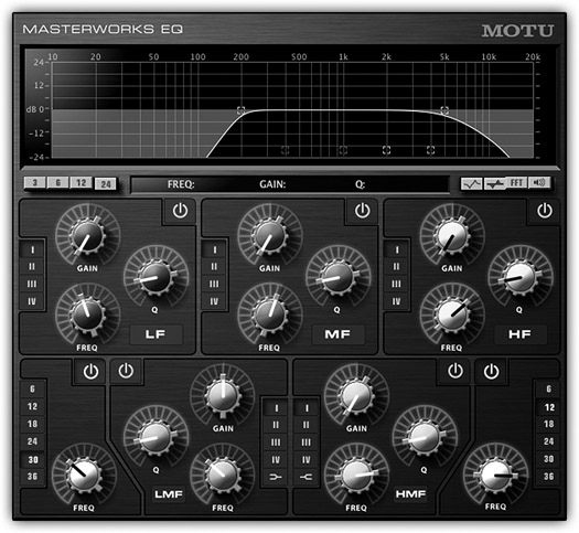
Figure 15.31 An HPF and LPF combined to form a band-pass response (the MOTU MasterWorks EQ). The two filters are set to remove frequencies below 200 Hz (HPF) and above 5 kHz (LPF). Band-limiting instruments in a similar way can increase separation and reduce masking.

The general idea is to restrict an instrument to a limited band, which can increase separation. One example of where this can be beneficial involves distorted guitars. These often have an excess of both low-end rumble and high-end noise. Being forceful maskers as they are, band-limiting them also reduces their masking interaction to a limited range of frequencies. Other instruments can also benefit from such an approach.

Shelving filters

While both pass and shelving filters affect the extremes, pass filters remove, while shelving filters soften or emphasize. Needless to say, a shelving filter can boost and a pass filter cannot. One important characteristic of shelving filters is that they are not as aggressive as pass filters—while with shelving filters we have ultimate control over the gain amount, with pass filters we get the less flexible slope control. Shelving filters can be set to have very little effect and their response curves are generally gentler.

The various applications of pass filters can easily become a shelving job if we exchange the word “remove” for “soften.” For example, sometimes we only want to soften the body of vocals, not get rid of it altogether. Sometimes we want to reduce the size of a reverb, but still keep some of its warmth. The high-frequency noise on distorted guitars might only call for moderating. Sure enough, we can always use a combination of pass and shelving—pass to remove unwanted content (e.g., rumble), shelving to soften wanted content (e.g., body).

Shelving filters are often associated with the terms thick and thin (for the lows), and bright and dark (for the highs). We are all familiar with the shelving effect from our hi-fis. Having the same ability to shape the tonality of each individual instrument is a great asset. Two key challenges that the frequency domain involves are balanced spectrum and separation between various instruments. Referring back to Figure 6.2, it was suggested that we take an abstract approach and imagine where each instrument is located on the frequency spectrum, how wide it is, and whether there are any lacking frequency ranges in our mix. In the journey to balance spectrum and separation, we might want to nudge various instruments up or down on the frequency spectrum. We might also want to narrow or widen their frequency range. This practice is often referred to as tuning an instrument into the frequency spectrum. Keeping the same abstract approach, we could really use the ability to nudge the lower or higher boundary of an instrument.

Shelving filters are great tools for doing this, and Figure 15.32 illustrates how. Essentially, if you want an instrument to take more of the highs, boost using high shelving; if you want it to take less, attenuate. Using the very same principle, if you want an instrument to take more of the lows, boost on a low shelving; for less of the lows, attenuate. The only trick is to hit the right shelving frequency. The advantage that shelving filters have over pass or parametric ones is that they can be set for a very subtle effect (unlike pass) and affect a wide frequency range with a flat response (while parametric are more oriented toward a specific range of frequencies).

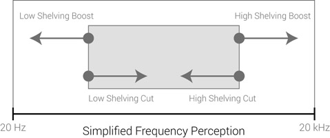
Figure 15.32 Tuning an instrument frequency range using shelving filters. Low shelving affects the low boundary: boost lowers it, cut makes it higher. High shelving affects the high boundary: boost makes it higher, cut lowers it.

Parametric filters

Parametric filters are used when we wish to treat a specific range of frequencies. Often these specific ranges are associated with some spectral component of the treated instrument (e.g., body) or with a general sonic quality (e.g., nasal). Although not limited to the midrange, often this is the range parametric filters treat.

Recognizing and comprehending the essence of various frequency ranges takes a lifetime of experience. A popular trick can help us locate the right frequency when using parametric filters. Say we are trying to find the attack of a kick. The technique involves a generous boost with a narrow Q, then sweeping the center frequency across the spectrum. The frequency at which the kick’s attack is most profound is the frequency we are after. Then, we adjust the gain and Q. While many mixing resources mention this technique, it has some strong opposition as well. For one, it hinders critical evaluation skills, which are based on the process of listening, analyzing, then taking action. It can be compared with the less experienced guitarist playing all sorts of possible chords in the search for the right one. Then, there is the same risk of liking the boost too much, and ending up with a higher gain than appropriate. Having said that, this technique can still be helpful for the less skilled engineer and with tricky material.

Although gain settings are often straightforward, even here there is more than meets the eye. We have already discussed the upward vs. sideways principle, where we demonstrated that gain can sometimes be traded for Q. How much effect an equalizer has is a function of both the gain and Q settings. Perhaps surprisingly, exactly the same settings and response curve on two different equalizers might not produce identical results. While the gain on an equalizer can have a noticeable effect with 0.5 dB of boost, certain equalizers offer up to 18 dB of gain. A 15 dB boost could be harrowing, but it can also be musical. For these reasons, it is not easy to generalize what typical gain settings are—it depends on many factors such as the frequency, Q, source material, and equalizer being used. Some people regard 1 dB as gentle, 3 dB as conservative, 6 dB as moderate, 9 dB as serious, and 12 dB as extreme.

Figure 15.33 Harmonics equalization. (a) Standard equalization, where a single range of frequencies is equalized. (b) Harmonics equalization, where the same range is equalized with a softer response, but its harmonic is also equalized.

One useful equalization technique involves distributing the equalization load across different frequencies. More specifically, instead of equalizing around one frequency only, we also equalize around its harmonic (an octave above). Figure 15.33 demonstrates this. This lets us reduce the gain on the first frequency and shift that gain to the harmonic. Compared to using one band only, each of the two bands will have a less drastic response and less phase artifacts. Also, having the equalization take place at two points often has the advantage of overcoming masking.

Q settings are also a vital part of equalization. A Q too wide might take on board unrelated frequencies, whereas a narrow Q might not be effective enough. Narrow Q is often used when we want to treat a very narrow bandwidth, often an unwanted noise or a resonant frequency. Wide Q tends to sound more natural and is mostly used to emphasize wanted parts of the frequency spectrum and for fine tonal alterations. Accordingly, wide Q is more common with boosts and narrow Q with cuts.

Spectral components

We say that we can divide the timbre of each instrument into four parts: lows, low-mids, high-mids, and highs. Learning how each of these bands affects the tonality of an instrument is one of the first things mixing engineers should grasp. It only takes a few minutes to experiment with how each band affects the tonality of an instrument—the experience is invaluable. However, the equalization of each instrument is not as simple as that— subtle alteration of very specific frequencies can have a dramatic effect. By way of analogy, the equalization of each instrument is like a safe waiting to be cracked. It would be fair to make no subdivisions at all—it is simply 20 Hz–20 kHz and what we are after can be anywhere. Once familiar with the four different bands, we progress and learn how smaller ranges affect the timbre of various instruments. Each instrument has a few influential spectral components—frequency ranges highly vital for its timbre. Learning these takes a bit more time as different instruments have different spectral components at different ranges.

The rest of this chapter covers common instruments, their spectral components, and other frequency ranges that might be of interest to us.

Vocals

It can be argued that the term vocals alone cannot encompass the great variety of human voices. For one, the voices of males and females are different. Then, each person has so many unique qualities in his/her voice that every singer can be considered a completely different instrument. It should be fair to assume that vocal equalization starts by eliminating the wrongs—the likes of muddiness, honky sound, and sibilance if apparent (which deessers are likely to rectify better). Being the key element of many productions, vocals must be most prominent. It is vital for vocals to overcome any instrument that masks them. This might entail equalization not only on the vocals, but also on the masking instrument. Different vocal parts have different roles in mixes, so at times we make them sweet, at times warm, and at times aggressive. Generally speaking, the more powerful the vocal part is, the more equalization will be used.

Figure 15.34 shows the possible frequency range of the human voice. The long gradient bar shows the possible frequency content of both fundamentals and harmonics. The bounded rectangle denotes the possible fundamentals range, which ranges between 82 and 1,398 Hz (E2–F6). No person can produce this full range of notes. Also, the extremes of this range can only be produced by skilled opera singers. To give an example, Mariah Carey’s vocal range spans approximately 123–830 Hz (B2–G#5). Typical pop singers cover a far less impressive range than that. Above and below the bar are frequency ranges relevant to vocals. It is worth noting that equalizing a specific range can yield either positive or negative results. For example, by boosting the high-mids we might add presence, but at the same time add unwanted sibilance. By attenuating the low-mids we might add clarity, but lose warmth and make the sound thin.

Figure 15.34 The frequency range of the human voice and relevant frequency ranges. The gradient bar denotes the range of possible fundamentals and harmonics. The possible fundamental range is confined in a rectangle. The associations above the bar are likely to be emphasized by a boost in their frequency ranges, the associations below by a cut.

Overheads

The overheads glue all the individual drums together. When the overheads are too quiet, the drums can sound very artificial and come across as lifeless. There are three general approaches to the involvement of overheads in mixes. What differs from one approach to the other is the amount of low-end filtering in combination with the overheads level:

• Main stereo pair—the overheads are responsible for the majority of the drum sound, with possible minor reinforcement from close-mics, mostly kick and snare. This is typical in conventional jazz mixes and more natural-sounding productions. No or subtle low-end filtering is applied.
• First among equals—an equal share between the overhead and the close-mics. This is common in contemporary productions where kicks and snares are very prominent. An HPF might be positioned in the frequency range between the kick and the snare, mostly to clear the low-end for the kick’s close-mic and reduce spatial cues that send the various drums backward.
• Cymbals only—the overheads are responsible for the cymbals only, and the close-mics for all other drums. This least-natural approach entails strong high-pass filtering (even into the high-mids), intended to remove as much drum content (and room) as possible. This technique can be a lifeboat when the overheads are seriously flawed—nothing new in low-budget and home recordings.

In addition to the drum kit itself, overhead recordings also include the room response (the reverb). This creates an illusion of space in the mix, which is more or less similar to that of the recording space. The problem is that sometimes there is too much room, sometimes the space is just not appealing—most domestic rooms and even some studio spaces can produce a weary mix ambiance. HPFs let us correct, to some extent, such recordings.

The size, depth, and impression of reverbs focus on their lows. One particular problem is that low-frequency drums, notably the kick, tend to excite most rooms more than, say, the cymbals. This is normal as low frequencies take longer to absorb. Yet, it is a definite attribute of overheads recordings due to the small live rooms often used. As an outcome, the reverb from the overheads imposes some depth on the kick, toms, and the snare. Such depth might be unwanted, and, no matter how the close-mics are mixed, it can be hard to get the drums to the in-your-face position. Filtering the lows from overheads reduces spatial information and helps bring the individual drums forward in the depth field. The more we filter, the smaller we make the room and the closer the image becomes. In order to eliminate more of the individual drums but retain more of the cymbals’ timbre, a steep filter is often needed. Combined with the fact that overheads are a broadband signal that involves transients, a high-quality HPF is a requisite for the task. For more gentle results, a shelving filter can be used instead of a pass filter—it allows us to keep more of the warmth and spatial impression that the overheads contribute, but still reduces their size and depth contribution.

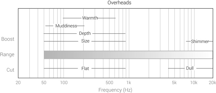
Figure 15.35 The frequency range of overheads and relevant frequency ranges.

By taking the cymbals-only approach, we can filter a flawed room from the overheads. If this dries out the mix ambiance, we can always use a technique called ambiance reconstruction—sending the individual drums into a reverb emulator to recreate the missing ambiance. We have full control over the reverb we choose, but we have to make sure that it matches the high-frequency reverb still present on the overheads.

Unless recorded in a good room, the low end of the overheads might muddy the mix. Both the lows and low-mids can benefit from some attenuation that will clear some space for the kick (close-mic), bass, and the fundamentals of other instruments. However, caution must be taken as the same lows might contribute to general warmth and the sense of ambiance in the mix.

The highs of the overheads contribute some shimmer. If no cymbal mics are mixed, the overheads might be the ones to govern the high-end of the mix. Thus, how bright or dull we make the overheads can also govern how bright or dull the mix is, and in turn how balanced the overall mix is.

Kick

If you listen to a collection of productions, you will find kicks in many shapes and forms— the thunderous, the rounded, the 909, the 808, the woody, the typewriter style, the basketball, the pillow-like, to name a mere few. How we shape the sound of a kick is often part of creative decisions we make; we control aspects such as solidness, punchiness, thickness, and snappiness. But the sound of the kick is also a practical affair. Being the admiral of the rhythm, the kick has immense weight in the ability of the mix to move people. A weak kick on a hip-hop mix means a weak hip-hop tune; ditto for dance; and mostly so for rock, pop, and metal. When it comes to mixing kicks, equalizers play a powerful role.

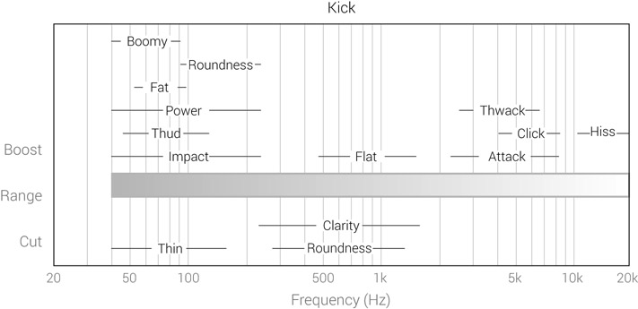
Figure 15.36 The frequency range of a kick and relevant frequency ranges.

Kicks have two main spectral components—the impact and the attack. These two components correspond closely with the lows and high-mids, respectively. Within these two ranges, different frequencies have a different effect. For example, 60 Hz might produce more oomph, while 90 Hz might produce more thud. Dance and hip-hop might benefit from robust oomph, while rock and pop might benefit from a solid thud. On the high-mids, the higher the frequency, the more the click. A healthy boost around 8 kHz can produce the typewriter click that many associate with heavy metal. The low-mids of the kick could have little to offer, and attenuating them can clear useful space for the low-order harmonics of other instruments. On the highs, kicks have very little valuable energy, which is sometimes entangled with hiss. Rolling off the highs from a kick could go unnoticed.

One important aspect of equalizing a kick is how it interacts with the bass. As the two instruments are competing for the lows, sometimes we have to sacrifice the impact of one for the benefit of the other. Another important issue with mixing kicks is that there is always a risk of mishandling the low-end due to limited monitors or poor acoustic environments. Under such conditions, it pays to spend some time going through the stabilizing options described in Chapter 4.

Snare

Perhaps the prince of rhythm, the tonality of the snare is also an important aspect of many mixes. Snare recordings are not always ideal. It is often only high-budget projects that can afford snare comparisons, fresh skins, accurate tuning, appropriate muffling, a suitable microphone, and correct placement. In all other projects, snares are prone to a few issues that might need correction—excess rattle and resonant ring are two such examples.

Although the spectral components of a snare are not as distinct as those of a kick, we often talk about body and presence, while also considering aspects such as snap and crispiness. A part of snare mixing entails tuning them into the frequency spectrum; that is, deciding how high or low they sit, also with relation to other instruments. A dark snare will be more distant and laid back. A bright snare will be more upfront. Automating snare sounds (between verse and chorus, for example) has rationale in more than a few mixes.

Figure 15.37 The frequency range of a snare and relevant frequency ranges.

Toms

While often only playing occasionally, toms might just be blended into the overall drum sound, but can also be mixed to have a distinct powerful impact. Toms, notably floor toms, can get a bit out of control unless we contain their lows. Also, it is important to observe timbre differences between the various toms—poorly tuned toms that are recorded with different microphone brands can sound as if each belongs to a different kit.

Toms have some similarity to kicks in the way we mix them, but they have more defined pitch and longer decay. Unsurprisingly, a high tom will have its spectral components higher on the spectrum than a floor tom. At the very lows, there is usually rumble that might need filtering. The fullness and thud are around the higher lows, 200 Hz or so. The attack, as with kicks, is on the high-mids. It is also worth seeing whether cutting the highs reduces cymbal spill without affecting the sound of the toms.

Figure 15.38 The frequency range of toms and relevant frequency

Hi-hats and cymbals

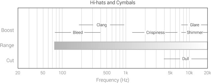
Figure 15.39 The frequency range of hi-hats and cymbals, and relevant frequency ranges.

The hi-hats are often the brightest element constantly playing in the mix. As such, they could play a big part in our perception of how bright the mix is altogether. One common problem with hi-hats is that they sound detached from the rest of the mix. To elaborate, they are perceived in the spectrum as the brightest instrument, but there is some empty frequency range below them. This is often the outcome of overemphasized highs. One characteristic of many pleasing mixes is that the hats are not glaring bright—they just shimmer. It is worth remembering that it might be the overheads contributing to this aspect in the mix and not close-mics.

Cymbals have very similar characteristics to hi-hats, but as they only play occasionally they play a less crucial part in the overall frequency balance. The larger the cymbal, the lower is its fundamental. Hi-hats, for example, can have some content below 500 Hz; rides go lower than that. These lower ranges of cymbals, which often involve bleed, can sometimes be pulled without affecting too much of the timbre.

Bass

Usually one of the trickiest instruments to mix is the bass—whether a guitar or a synth. For one, recordings tend to be very different from one another. But the real problem with bass sounds is that their tone often changes in relation to the note being played. For example, the lower E (41 Hz) produces substantially more low frequencies than the E two octaves above it (164 Hz). Solid tone can be achieved with equalizers, although both dynamic equalizers and compressors (especially multiband) can do a better job. There are also different playing techniques and different bass sounds in different genres. The bass in funk, for example, is miles away from the bass in metal.

There are two principal aims when mixing a bass: power from solid lows, and definition. Neither is easy to achieve. Being of a sustained nature in most productions, the bass is often the instrument that fills the low-end. Too many lows and the mix is boomy; too few and the mix is thin (and, as mentioned, this characteristic can change in relation to the note being played). Then, the bass and the kick often compete for the lows. Most bass sounds have relatively little energy on the high-mids and highs, and some have no energy at all above, say, 5 kHz (specific recordings can have almost nothing even below that). On the low-mids, there are usually enough instruments fighting for space. So defining the bass might require some experimentation. Any mixing tool that generates harmonics (distortions and enhancers, for instance) can be extremely useful in providing some definition for bass sounds.

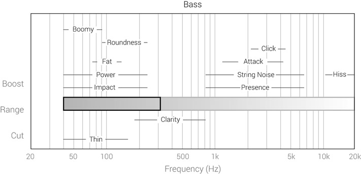
Figure 15.40 The frequency range of a bass guitar and relevant frequency ranges.

Acoustic guitar

Acoustic guitars can play various roles in the mix. On some mixes, often sparse ones, the guitar is one of the main instruments, usually along with the vocals. In such circumstances, we often want the guitar sound to be rich and full-bodied. On other mixes, the acoustic guitars only provide a reinforcement of the harmony and rhythm, which means that their body is less important. Very commonly acoustic guitars are treated with HPFs. The cutoff frequency is set depending on how much space there is, often starting from around 80 Hz—just below the lower E (subject to standard tuning). In many commercial mixes, the body of the guitar is fully removed, leaving it playing more of a rhythmical role than a harmonic one. When appropriate, the cut-off frequency is set so high that all that is left is a very thin, somewhat metallic sound—the played chords can hardly be discerned.

Another aspect of equalizing an acoustic guitar involves treating its body resonance, which could result in the unwanted accent of a specific spectral area or an increased level and sustain of specific notes. Finger squeaks are another thing we might want to reduce (or accent) using equalization. We can also control the timbre of the guitar by accenting or easing second- and third-order harmonics, which are found on the low-mids. The very highs of an acoustic guitar can be very sensitive to boosts, and even a small push from 10 kHz and above can make the sound appear thin and cheap. For this reason, if an acoustic guitar needs to be brightened, it could benefit from a wide-Q bell, rather than a shelving EQ.

Figure 15.41 The frequency range of an acoustic guitar and relevant frequency ranges.

Clean electric guitar

Electric guitars are an inseparable part of rock music, and on many productions provide the harmonic backbone. Most of them arrive at mixing stage already equalized—whether by the tone controls on the guitar itself or those on the amplifier. Often our aim with clean electric guitars is making them well defined, yet without masking other instruments. The way the guitar is played is a factor in the way it is mixed. Some involve strumming chords while others are played in a phrasal fashion; some are played more rhythmically while others more melodically. The latter require more attention for spectral balance between different notes. Often we get more than one guitar, and, unless different on the recordings, we can distinguish them using equalization. Although to a lesser degree than with acoustic guitars, electric guitars can also benefit from low-end filtering, which is dependent on the density of the arrangement.

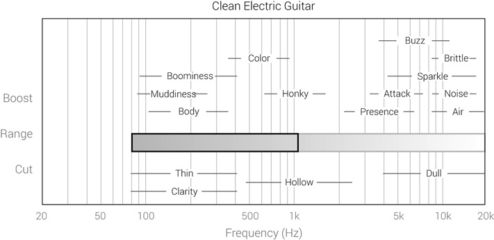
Figure 15.42 The frequency range of a clean electric guitar and relevant frequency ranges.

Distorted guitar

Perhaps the frequency-richest instrument is the distorted guitar. This is both a disadvantage and an advantage. It is a disadvantage since distorted guitars are masking animals—most of them have dominant energy from the very lows to the very highs, and they can easily cloud everything else. It is an advantage since we can shape their sound in many fascinating ways. Distorted guitars are super-EQ-sensitive. A boost of 3 dB on the high-mids can easily make an EQ whistle. They are responsive all the same to small level cuts. A quick listen to commercial tracks reveals that many distorted guitars are elegantly powerful, but not pushily powerful. Put another way, they are not just thrown into the mix at a loud level, but crafted more wisely to blend with other instruments. In many cases, distorted guitars also involve some stereo effects.

Figure 15.43 The frequency range of a distorted guitar and relevant frequency ranges.

Low-end rumble is often removed or attenuated. How much and up to what frequency the filter goes is done by ear. It is worth remembering that we can first clean the mix (going a bit higher with the filter) and later add a few more lows if we still feel these are missing. Much of the sound of distorted guitars has to do with the actual distortion being used, and there are as many flavors of guitar distortions as there are notes on a guitar. Often the high-end contains grainy noise that the mix can live without. The mids can also benefit from softening, which generally clears some space for all the other instruments. But taking too much of the mids creates a very distant sound that is mostly associated with some metal subgenres. Another consequence of softening the mids is that the guitars become louder as the mix is played louder. This is the nature of any instrument with pulled mids, but it makes more sense with distortion guitars since they are more controlled in quiet levels but emphasized at louder levels (where things tend to get messier anyway).