
24
Reverbs
With the exception of pure orchestral recordings, reverbs are used in nearly every mix. The common practice of close-miking and the dry nature of some sounds produced by synthesizers and samplers result in initial mixes that lack both ambiance and depth (such mixes are often described as “2D mixes”). Reverbs allow us to add and build up these missing elements during mixdown, but they can also be beneficial for many other mixing tasks.
What is reverb?
In nature, reverb is heard mostly within enclosed spaces, such as rooms. Reverbs are easier to understand if we imagine an impulse sound, such as a handclap, emitted from a sound source in an empty room. Such a sound will propagate in a spherical fashion, and for simplicity we should regard it as traveling in all directions. The emitted sound will travel in a direct path to a listener (or a microphone) followed by reflections that bounce from the walls, floor, and ceiling. These will gradually be followed by denser reflections that have bounced many times from many surfaces. As sound diminishes both when traveling through air and being absorbed by surface materials, the reflections will slowly decay in level. Reverb is the collective name given to the sound created by bounced reflections from room boundaries (which we consider to be the main reverb contributors, although in a room there might be many surfaces). In mixing, we use reverb emulators, either hardware units or software plugins, to simulate this natural phenomenon.
Applications
Simulating natural or creating imaginary ambiance
Due to the inflexible nature of ambiance recordings and the poor reverb characteristics of many live rooms and home studios, many engineers choose to record most instruments dry and apply artificial ambiance during mixdown. While mixing, reverb emulators give us more options and control over the final ambiance of the mix.
Creating the ambiance of a production is considered one of the more important and challenging practices in mixing—ambiance transforms a collection of dry recordings into an inspiring spatial arrangement that gives our mix much of its character. The reverb controls let us mold the ambiance and make creative decisions that can make our mix more cohesive and vigorous.
Many regard the creative process of crafting ambiance a vital part of mixing.
Here again, we have a choice between a natural or unnatural (or imaginary) outcome. A natural ambiance is expected in some mixes and for some genres; jazz, bossa nova, and productions that include an orchestral performance, for example. For such projects, we might choose to utilize natural reverb simulations so that the listener can conceive the performance as if being played in a very familiar type of space. Realism is obviously an important factor in natural simulations—not only is the reverb choice important, but also the way we configure it to support the depth of individual instruments and the different properties of the simulated space.
While we can imagine the typical ambiance of a jazz performance, what ambiance should we employ for a trance production? How about electro, hip-hop, trip-hop, techno, or dubstep? There is a loose link between sequenced productions and acoustic spaces. For such projects, the ambiance is realized based on the creativity and vision of the mixing engineer. Furthermore, sometimes an imaginary ambiance is applied even when a natural one is expected. This is done in order to achieve something refreshing, different, and contemporary. Such implementation is evident in some recent jazz albums that, in addition to unnatural ambiance, utilize many modern recording and mixing techniques.
An important point to remember is that while selecting an ambiance reverb, we might ask ourselves, “How attractive is this reverb?” and “How well does it fit into the mix?” rather than dealing with the question of, “How natural?” Such thinking promotes less natural reverbs, and we have already discussed how a nonnatural mix can bring about a fantastic result—an imaginary space can excite us more than the familiar, natural ones.
While a natural choice might be suitable for some productions, an imaginary ambiance can sometimes be more rousing and effective.
Gel the instruments in the mix
After combining the various tracks, each instrument in the mix might have a distinctive appearance, but heard together they might feel a little foreign to one another—there might be nothing to link them. A reverb, even one that can hardly be perceived, can gel the various instruments, making them all appear as a natural part of the mix. Similarly to ambiance reverbs, one emulator might have many tracks sent to it, but, in contrast to ambiance reverbs, the gelling reverb is more subliminal: it might not be audible or have a clear spatial sense, and will be felt rather than heard.
Increase the distinction of instruments
Although we have just advocated sending many instruments to the same reverb, different reverbs on different instruments can sometimes be beneficial. For example, having the guitars feeding a specific reverb and the vocals feeding another, despite creating a less natural space, would increase the distinction between the two instruments, resulting in increased separation.
Depth
In nature, many factors contribute to our perception of depth. The natural reverb in a room is key. During mixdown, reverbs are the main tool we use when positioning sounds in the depth field. This is extremely desirable in many situations—it adds another dimension to the mix, lets us position instruments more naturally, establishes hierarchy, and can also help with masking. But the bond between depth and reverbs does not come without a price—the perceived depth caused by the addition of reverb is sometimes unwanted, for example when adding reverb to vocals while still wanting to keep them in the front of the mix.
Although sometimes unwanted, reverb addition often increases the perceived source-to-listener distance, and therefore reverbs are regularly utilized for applying depth.
Enhance a mood
Different productions have different moods—happy, mellow, dark, and aggressive are just a few examples. Reverbs are often associated with tenderness, romance, mystery, intimacy, and many other sensations and atmospheres. We can enhance, and even establish, a production mood by using reverbs creatively.
Some genres, such as chill-out and ambient, embrace reverbs as a production means. But while reverbs are usually more evident in slow productions, it is perhaps the spatial disorientation caused by certain drugs that fosters reverb use in some upbeat dance genres (and psychedelic music in general).
Livening sounds
Those who have heard a recording that took place in an anechoic chamber or those who have attended an unamplified performance in an open field know how unsatisfying such a reverb-free performance can be. Reverb is a native part of our life as it accompanies most of the sounds we are exposed to. A reverb-free recording of specific instruments, as good as it may be, can sound cold and unnatural. By adding reverb, we take a dry, artificial recording and breathe “life” into it—adding the reverb we are so familiar with in daily life.
However, it is not only the existence of a reverb that matters—it is also the amount of reverb. Ask yourself whether you like your singing better when “performing” in your bedroom or in your bathroom. Most people will choose the latter since mostly it has a louder and longer reverb. Reverbs can make sounds more impressive and more present; when we say “livening,” we also mean taking a stodgy performance and turning it into a captivating one.
Another issue that comes to mind here is the use of mono samples in sequenced production. For instance, a mono ride sample can sound odd compared with the familiar sound of a ride captured by stereo overheads. Adding reverb to mono samples can produce a more natural and less mechanical feel to sequenced instruments.
Filling time gaps
Empty time gaps can break the balance and integrity of our mix. Reverbs can make mix elements longer and fill empty time gaps, an application more common in slow, sparse productions.
Filling the stereo panorama
Consider a slow production consisting of an acoustic guitar and vocal recordings only. How can one craft a full stereo panorama with just two instruments? Stereo reverbs can be utilized in mixes to create an imaginary sound curtain behind the performers. Often reverbs of such type span the stereo panorama. But we can also use reverbs to fill gaps in the stereo panorama by simply padding specific instruments with a stereo reverb, making their stereo image wider.
![]()
Track 24.1: Guitar Dry
The source guitar track, dry, with its focused and thin image at the center of the panorama.
Track 24.2: Guitar with Reverb
The added reverb fills the stereo panorama. Also, notice that the guitar appears farther back although the level of the dry signal has not changed.
Plugin: Universal Audio DreamVerb
Changing the timbre of instruments
In many situations, added reverbs modify the timbre of the original sound, whether it be our desire or not. A loud reverb on a percussive instrument can smoothen its attack, slow its decay, or create a completely different decay envelope. The friction between a violin string and a bow can produce a harsh noise that can be blurred and softened by a reverb. Conversely, though, it is exactly that friction noise that can give a double bass added expression in the mix. A reverb can be used to constructively alter timbre, but it can also deform it (a possibility we must be aware of). In most situations, the right reverb choice along with appropriate control adjustment will render the desired result.
When adding reverb, we listen closely to timbre changes and, when needed, tweak the reverb parameters.
Reconstruct decays and natural ambiance
Reverbs can also be used to replace the natural decay of an instrument. Such an application might be required if a tom drum recording contains exaggerated spill. Toms are commonly compressed in order to give them more punch and bolder decay, but doing so will also amplify the spill, which can cause some level fluctuations in the mix. To solve this, we gate the toms so the decay is shortened, then feed the gated tom into a reverb unit, which produces an artificial decay. We have much more control over artificial decays and we can, for example, make them longer and bigger, so as to make the toms prominent.
A similar application is the reconstruction of room ambiance. A classic example is the ambiance captured by a pair of overheads. It can be very tricky to control such ambiance and fine-tune it into the mix, mainly with regards to frequencies and size. It can become even more problematic after these overheads tracks are compressed, since this will emphasize the ambiance even more. The low and mid frequencies, where most of the presence and size of the ambiance are found, can be filtered and reconstructed using a reverb.
![]()
Track 24.3: Drums Before Reconstruction
These are the original drums, unprocessed.
Track 24.4: Drums After Filtering
Only the room and the overheads are filtered in this track. A 12 dB/oct HPF at 270 Hz removes much of the ambiance. The drums now sound thinner and their image appears to be closer.
Track 24.5: Drums After Reconstruction
The close-mics are sent to a reverb emulator, which is preceded by an LPF. The result is ambiance different in character from that in Track 24.3.
Plugin: Audio Ease Altiverb
Drums: Toontrack EZdrummer
Resolve masking
Although a potential masker in its own right, a reverb can be used to resolve masking. The common usage of reverbs for the purpose of depth gives us the ability to position sounds in a front–back fashion, in addition to the conventional left–right panning. This adds another dimension and much more space in which we can place our instruments.
A stereo reverb, which spreads across the sound stage, has more chance of escaping masking, and its length means that it will have more time to do so. Say we have two instruments playing the same note and one completely masks the other. By adding reverb to the masked instrument, we make it longer and are able to identify it more because of its reverb.
More realistic stereo localization
Sounds that are not accompanied by reflections are very rare in nature. Panning a mono source to a discrete location in the stereo panorama can therefore produce an artificial result. Reverbs can be added to mono signals in order to produce more convincing stereo localization. The reverb will also extend the stereo width of the mono signal, which can make it clearer and more defined. The reverbs that are used for such tasks must be stereophonic and rely on a faithful early reflection pattern, and are usually very short.
A distinctive effect
Sometimes reverbs are added just to spice things up and add some interest. Snare reverb, reversed reverb, gated reverb, and many other reverbs are simply added based on our creative vision and not necessarily based on a practical mixing need. Reverbs can be automated between sections of the production in order to create some movement or be introduced occasionally to mark transitions between different sections.
Impair a mix
Although not exactly a constructive application, it is worth looking at the common problems that reverbs might cause and what we should watch out for:
- Definition—reverbs tend to smear sounds and to make them unfocused and distant, and can decrease both intelligibility and localization. Proper configuration of a reverb emulator can usually prevent these problems.
- Masking—as they are usually long, dense, and wide sounds, reverbs can mask other important sounds. As with any case of masking, mute comparison can reveal what and how reverbs are masking.
- Clutter—if used unwisely (which usually means too loud and for too long), reverbs can clutter the mix and give a “spongy” impression. Part of the challenge is making reverbs effective without being dominant.
- Timing—as a time-based effect, a reverb can affect the timing of a performance, especially a percussive one.
- Change timbre—discussed previously.
Types
Stereo pair in a room
The early method of incorporating reverbs into a mix (long before the invention of reverb emulators) was by capturing the natural reverb using a set of microphones in a room. Producers used to position musicians in a room in relation to how far away and how loud they should appear in the mix. Back then, and even today, different studios are chosen based on their natural reverb characteristics. In some studios, special installations, such as moving acoustic panels, are used to enable a certain degree of control over the reverb.
In most situations where a small sound source is recorded, say fewer than 10 musicians, the ambiance and depth of the room are captured by two microphones positioned using an established stereo-miking technique. As already discussed, such a stereo recording results in what can be described as a submix between the instrument and its reverb, which can be altered only slightly during mixdown. However, the celebrated advantage of this method is that it captures the highest extent of complexity that a natural reverb offers. No reverb emulator has the processing means to produce such a faithful, and natural, simulation, especially not in real time. As acoustic instruments radiate different frequencies in different directions, a microphone in close proximity can only capture parts of the timbre. But all radiated frequencies reflect and combine into a rich and faithful reverb, which is then captured by the stereo pair.
The reverb and depth captured by a pair of microphones in a room are the most natural and accurate ones, but they can be seriously limiting if they do not fit into the mix.
Reverb chambers (echo chambers)
A reverb chamber is an enclosed space in which a number of microphones are placed in order to capture the sound emitted from a number of speakers and the reverb caused by surface reflections. Either purpose-built or improvised, these spaces can be of any size and shape. Even a staircase has been utilized for such a purpose. A send from the control room feeds the speakers in the reverb chamber and the microphone signals serve as an effect return. While reverb chambers are generally not an accessible mixing tool for most engineers, every studio can be used as a reverb chamber—all studios (live rooms) have microphone lines and many have loudspeakers installed with a permanent feed from the control room.
The advantage of using reverb chambers is that the captured reverb is, again, of a very high quality, being produced by a real room. As opposed to a stereo recording, in which most mixing elements are immovable, reverb chambers are used during mixdown and provide more control over the final sound. This is achieved either by different amounts of send and return or by physical modifications applied in the chamber itself; for example, changing the distance between the microphones and the speakers or adding absorbent (or reflective) materials. However, such alterations result in a limited degree of control, and most of the reverb characteristics will only vary by insignificant amounts, most notably the perceived room size. We consider each reverb chamber as having a very distinctive sound that can only be “flavored” by alterations. Moreover, the loudspeakers used in a reverb chamber differ substantially from a real instrument in the way they produce and radiate sound, so reverb chambers are just a simple alternative to placing a real instrument in a real room. Another issue with reverb chambers is their size—a general rule in acoustics is that larger rooms have better acoustic characteristics than smaller ones. A small reverb chamber can produce a reverb with broken frequency response and reflections that can color the sound. A large reverb chamber is expensive to build and only big studios can afford it.
![]()
Track 24.6: Vocal Chamber Convolution
A chamber reverb simulation produced by a convolution emulator.
Plugin: Trillium Lane Labs TL Space
Spring reverb
Since reverb is essentially a collection of delayed sound clones, it is no wonder that one of the first artificial reverbs to be invented had its origins in a spring-based delay device. The original device was conceived by Bell Labs researchers who tried to simulate the delays occurring over long telephone lines. The development of the spring reverb, starting as early as 1939, is credited to engineers from Hammond who tried to put some life into the dry sound of the organ. During the early 1960s, Leo Fender added Hammond’s spring reverb to his guitar combo and was followed by manufacturers such as Marshall and Peavey.
A spring reverb is an electromechanical device that uses a system of transducers and steel springs to simulate reflections. The principle of operation is simple: an input transducer vibrates with respect to the input signal. Attached to the transducer is a coiled spring on which the vibrations are transmitted. When vibrations hit the output transducer on the other end of the spring, they are converted into output signal. In addition, parts of the vibrations bounce back onto the spring then bounce back and forth between the ends. Such reflections are identical to those bouncing between “surfaces in a one-dimensional space” (technically speaking, a line, with its boundaries being its end points).
In reality, the science of a spring reverb is more complex than the above explanation, but these units are relatively cheap to manufacture and still ship today with many guitar amplifiers. Although spring reverbs do a pretty bad job in simulating a natural reverb, listeners have grown to like their sound. Furthermore, many digital reverb emulators fail to match the sound of a true electromechanical spring reverb, which explains why standalone rack-units are still in production. Such units will be fitted with very few controls and in most cases will have fixed decay and pre-delay times. (It is worth noting that pre-delay could always be achieved if a delay was connected before the reverb; however, it was not until the early 1970s that digital delays started replacing tape delays for such purposes.) Quiet operation and flat frequency response were never assets of true electromechanical spring reverbs, and they are known to produce an unpleasant sound when fed with transients. Therefore, spring reverbs are usually applied on the likes of pads and vocals, normally while only mixing a small amount of the wet signal.

Figure 24.1 The Accutronics Spring Reverb. Source: Courtesy of Sound Enhancement Products, Inc.
While spring reverbs are far from spectacular in simulating a natural reverb, the sound created by a true electromechanical unit can serve as an identifiable retro effect, especially if applied on guitars and other non-percussive instruments and sounds.
![]()
Track 24.7: Vocal Spring Convolution
A spring reverb simulation produced by a convolution emulator.
Track 24.8: Snare Spring Convolution
The snare on this track is sent to the same emulator and preset as in the previous track.
Plugin: Trillium Lane Labs TL Space
Plate reverb
If a spring reverb is considered a “one-dimensional” reverb simulator, the logical enhancement to such a primitive design was going “two-dimensional.” The operation of a plate reverb is very similar to that of a spring reverb, only that the actual vibrations are transmitted over a thin metal plate suspended in a wooden box. An input transducer excites the plate and output transducers are used to pick up the vibrations. In the case of plates, these vibrations propagate on its two-dimensional surface and bounce from its edges.
In 1957, a pioneering German company called EMT invented and built the first plate reverb— the EMT 140. This model, which is still a firm favorite, had the impressive dimensions of 8 ft × 4 ft (2.4 m × 1.3 m) and weighed around 600 pounds (more than a quarter of a ton). These original units were very expensive but still much cheaper than building a reverb chamber. They can be heard on countless records from the 1960s and 1970s and on other productions that try to reproduce the sound of these decades.
While mobility was not one of its main features, the plate reverb had better sonic qualities than the spring reverb. In addition to a damping mechanism that enabled control over the decay time, its frequency response was more musical. The reverb it produced, although still not resembling a true natural reverb and being slightly metallic, blended well with virtually every instrument, especially with vocals. The bright, dense, and smooth character of plate reverbs also made them a likely choice for drums, which explains why they are so frequently added to snares.
Although a serious artificial reverb simulator, a plate reverb does not produce a truly natural-sounding reverb. Hence, it is used more as an effect to complement instruments such as snares and vocals.
![]()
Track 24.9: Vocal Plate Convolution
A plate reverb simulation of the EMT 140 produced by a convolution emulator.
Track 24.10: Snare Plate Convolution
The same emulator and preset as in the previous track, only this time being fed with a snare.
Plugin: Trillium Lane Labs TL Space
Digital emulators
So far, we have discussed natural and mechanical reverbs. The invention of digital reverberation is credited to Manfred Schroeder, then a researcher at Bell Laboratories, who, back in 1961, demonstrated a simple digital reverberation system (Figure 24.2a). It took a while to turn his digital reverberation ideas into a tangible commercial machine, but with the performance rise of DSP chips and the fall in their price, digital emulators were destined to take over. It was EMT again, with help from an American company called Dynatron, that, in 1976, revealed the world’s first commercial reverb unit—the EMT 250. It consisted of very basic controls, such as pre-delay and decay time, and produced effects such as delay and chorus.
A digital reverb is not a dense collection of simple delays, since these would cause much coloration to the direct sound and produce a broken frequency response. There are many internal designs for digital reverbs and they vary in their building blocks and in the way these blocks are connected. At the lowest level, digital emulators are implemented using mathematical functions that are executed on internal DSP chips. To differentiate from digital convolution reverbs (discussed later), these types of reverbs are now referred to as algorithmic reverbs.
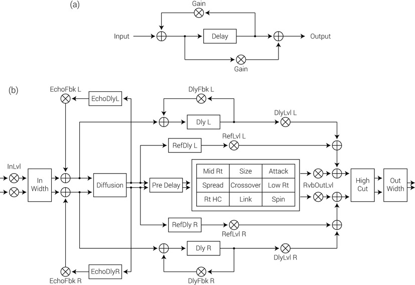
Figure 24.2 Block diagram of a reverb. (a) The original Schroeder reverb design (1961). Later digital designs are far more complex, as can be seen in (b): the plate program of the Lexicon PCM91 (1998).
![]()
Track 24.11: VocalEMT 250 Convolution
A plate reverb simulation of the EMT 250 produced by a convolution emulator. Notice that, compared to Track 24.9, this reverb has better spatial characteristics.
Plugin: Trillium Lane Labs TL Space
No digital emulator will ever be able to produce a reverb completely identical to the one created in a real room. This is mainly due to the complexity of such a reverb—there are thousands of reflections to account for; different frequencies propagate and diffract in different fashions; different materials diffuse and absorb sound in different ways; and even the air itself changes the sound as it travels through it. Manufactures must take shortcuts, and the more processing power is at their disposal the fewer shortcuts they have to take, and thus the more realistic the reverb is likely to be. It is worth noting that although DSP chips were far less powerful in the 1970s and 1980s, many units from these decades are still regarded today as state-of-the-art, which shows just how important the design of such units is. Since each respectable manufacturer has their own secret architecture, each has a distinctive sound.


Figure 24.4 The “larc” (lexicon alphanumeric remote control) for the Lexicon 480L; the reverb unit itself is rack-mounted and often unseen in studios. Despite being released in 1986, the 480L is still considered by many as one of the best reverb emulators.
Source: Courtesy of SAE, London.
Back in the 1990s, when real-time plugins emerged, CPUs had less than a tenth of the processing power compared with modern processors and could only handle a few plugins at a time. Today, more and more people rely solely on their computer CPU for all mixing tasks. Yet, a high-quality reverb plugin can consume significant amounts of the CPU processing capacity, so many still find the need for additional processing power—either in the form of external hardware units or as internal DSP expansion cards.
As algorithmic reverbs have no physical or mechanical limitations, they provide a multitude of controls that let us tweak nearly every property of the reverb. This makes them an extremely flexible and versatile tool in many mixing scenarios, and it is no wonder that they are the most common reverbs in our mixing arsenal. An issue with high-quality emulators is that they are expensive both in terms of price and processing-power consumption.
Digital reverbs are the most common type in use and give us great control over reverb parameters, but they can consume large amounts of processing power, depending on their quality.
Convolution (sampling) reverbs
Even back in the 1970s, various people toyed with the possibility of capturing the reverb characteristics of an acoustic space, so it could be applied later to any kind of recording. What may have sounded like a pipe dream has become a reality with the new millennium, with DSP technology now fast enough to accommodate the real-time number of calculations required for such a process.
Reverb sampling is normally done by placing a pair of microphones in a room, then recording the room response (i.e., the reverb) to a very short impulse, like that of a starter pistol. Since it is very hard to generate a perfect impulse, an alternative method involves playing a sine sweep through speakers instead. The original sound might be removed from the recording, leaving the reverb only. The recorded impulse response (IR) is then loaded into a convolution reverb, which analyzes it and constructs a huge mathematical matrix that is later used by the convolution formula. With every sound fed through the unit, a reverb very similar to that of the original space is produced.

Figure 24.5 A convolution reverb plugin, the Audio Ease Altiverb.
An emulator can be based on one of two types of convolution: either one that is done in the time domain (pure convolution) or one that is based on the frequency domain (convolution or Fourier-based). Each generates the same result, only in some situations one will be faster than the other. If pure convolution were used, an impulse response of 6 seconds at 44.1 kHz would require around 23 billion mathematical operations per second—equivalent to the processing power offered by a 2.2 GHz processor. It can easily be seen how such a process might be unwieldy in some situations. As a general rule, the shorter the original impulse response is, the less the processing needed would be.
Convolution reverbs experience increased popularity nowadays. They let us incorporate into our mix the reverb of many exotic venues and spaces. For the film industry, this is a truly revolutionary tool—engineers can record the reverb of any location and then apply it during post-production. For mixing, however, it is doubtful how much the reverb characteristics of the Taj Mahal can contribute to a modern rock production. Yet, the impulse recordings shipped with emulators include less exotic spaces that can be used in every mix. Many impulse responses can also be downloaded from the Internet; some are free. The quality of the impulse recording is determined by the quality of the equipment used, which is a vital factor if natural results are sought. It is generally agreed that a good impulse recording produces an extremely believable reverb simulation that matches (if not exceeds) the quality of the best algorithmic emulators.
Convolution reverbs are not only used to reproduce the reverb of acoustic spaces. Impulse responses of virtually any vintage unit, such as the EMT 140 or 250, are also available. Fascinating results can also be achieved if instead of loading a real impulse response one loads just a normal short recording.
One problem with convolution reverbs is that all the properties of the reverb, as captured during the recording process, are imprinted into the impulse recording and can be altered very little later on without some quality penalty. An example of this is the inability to change the distance between the sound source and the listener or the different settings used while a hardware unit was sampled. Many convolution reverbs include only limited numbers of controls that make use of simple envelopes and filters in order to give some degree of control over the reverb characteristics. But for more natural results, many reverbs ship with a variety of impulse recordings of the same space, each based on a different recording setup. Generally speaking, convolution reverbs produce the best simulations provided the original impulse response is unaltered by the artificial envelope and filter controls. This fact makes convolution reverbs, to some extent, a hit-and-miss affair—if the pure impulse response is right, it should sound great; if it isn’t, additional tweaking might make it more suitable for the mix, but not as great. As with algorithmic reverb, the initial preset choice is crucial.
Good convolution reverbs can produce exceptionally natural results, but they consume processing power and are normally inflexible.
Perhaps the irony of convolution reverbs is that now, after having them at our disposal, many find the old algorithmic reverbs far more interesting and suitable for both creative and practical tasks. Despite the fact that convolution reverbs are considered superior in simulating natural spaces, algorithmic reverbs are still favored for many other mixing applications.
![]()
The following tracks demonstrate various IR presets from the Logic Space Designer convolution reverb. It is for readers to judge how realistic and appealing each of these reverbs is. It is perhaps most interesting to observe how, despite hardly adding a noticeable reverb, the Wine Cellar track has an extra sense of space and depth compared to the dry track.
Track 24.12: Conv Source
The dry source track used in the following samples.
- Track 24.13: Conv Wine Cellar
- Track 24.14: Conv Wooden Room
- Track 24.15: Conv Drum Chamber Less
- Track 24.16: Conv Wet Bathroom
- Track 24.17: Conv Small Cave
- Track 24.18: Conv Music Club
- Track 24.19: Conv Concert Hall
- Track 24.20: Conv Canyon
- Track 24.21: Conv Roman Cathedral
Here are two sets of samples demonstrating the use of just a normal sample as an IR. The results are unnatural, but can be used in a creative context:
- Track 24.22: Conga IR
- Track 24.23: Conv Conga
- Track 24.24: FM Noise IR
- Track 24.25: Conv FM Noise
Plugin: Logic Space Designer
Reverb programs
Digital emulators can simulate a number of spaces; each will exist as a loadable program (preset). As there can be hundreds of programs, these are organized in categories.
A high-quality reverb emulator might implement a different algorithm for each category. The main categories are:
| Category | Description | Application |
|
|
||
| Halls | Large, natural-sounding, live spaces | Natural |
| Chambers | Simulate reverb chambers or spaces that have slightly less natural reverb behavior and a less defined size | Natural |
| Rooms | Normal rooms of different sizes | Natural |
| Ambiance | Concerned more with placing the sound naturally in a virtual space, caring less about the actual reverberation; most often an ambiance preset involves early reflections only | Natural |
| Plate | Plate reverbs | Effect |
The following categories are also common:
| Category | Description | Application |
|
|
||
| Studio | Simulate the reverb in a recording studio live room | Natural |
| Church/cathedral | These types of spaces might produce a highly impressive reverb for certain types of instruments, such as organs, but they generally result in poor intelligibility | Natural |
| Spring | Spring reverb | Effect |
| Gated | Nonlinear reverb (explained later) | Effect |
| Reversed | Rising reverb instead of decaying one (explained later) | Effect |
Some mixes are expected to present a more natural space than others. If seeking a truly natural space in the mix, hall, or room, presets can produce good results. If less-natural reverb is required, either chamber or ambiance might be used. Most ambiance programs are essentially the shortest and most transparent of all reverb programs. They excel at blending mono instruments into a spatial arrangement, without adding a noticeable reverb.
The choice of category is usually determined by two main factors. First, the size of the room should fit with the type of music. A classical recording or a chill-out production might use a large space such as a hall; a bossa nova or jazz production can benefit from a moderate-sized hall; while a heavy metal or trance production might make use of very small space simulations. Second, the decay time (or length) of the reverb should be relative to the mix density—a dense mix will suffer from long reverb tails that will cause masking and possibly clutter; in a sparse mix, longer decays can fill empty spaces.
For a truly natural space, hall and room programs can work better than chambers and ambiance. The room size and the decay time are the two main factors when selecting a reverb program.
Within each category, various programs reside. For example, the halls category might include small hall, large hall, vocal hall, and drum hall. As opposed to EQs and compressors, it is uncommon for a mixing engineer to program a reverb from scratch—in most cases, a preset selection is made and then altered if needed. Initially, choosing the right program for the mix will involve experimentation—many mixing engineers will focus on one or two categories and will try all the different programs within each; if different units are available, each of these might be tested as well. It is time well spent, especially when selecting one of the main reverbs in the mix. A reverb that sounds good when soloed might not interact well with the rest of the mix—final reverb selection is better done in mix context. With experiment comes experience, and after a while we learn which emulator and which program works best for a specific task. The factory settings of each program are optimized by the manufacturer based on studies and experts’ opinions; therefore, drastic changes to these settings can theoretically degrade the quality of the simulation. This makes the initial selection of an appropriate program even more important.
The selection of an appropriate reverb program is highly important and is a process worth spending time on.
When a reverb is used as an effect, an artistic judgment is required since there are no golden rules. Many use plate programs on vocals and drums; snares are commonly treated with a plate reverb or a gated one. For a more impressive effect, chambers or halls can work. Halls can also be suitable for orchestral instruments such as strings, flutes, brass, and the saxophone. Bass guitars are usually kept dry, and distorted electric guitars can benefit from a subtle amount of small-room reverb that will add a touch of shine and space. As the association between synthesized sounds and natural acoustic spaces is loose, chamber and ambiance programs might be more suitable in a sequenced production.
The above should merely serve as a guideline—the final choice of reverb program should be a result of experimentation and will vary for each individual mix.
![]()
The following tracks demonstrate various reverb programs. Reverb programs can vary noticeably between one emulator and another, so readers are advised to treat the following tracks as a rough sample.
Track 24.26: Vocal Dry
Track 24.27: Drums Dry
The source tracks used in the following samples.
- Track 24.28: Program Hall (Vocal)
- Track 24.29: Program Hall (Drums)
- Track 24.30: Program Chamber (Vocal)
- Track 24.31: Program Chamber (Drums)
- Track 24.32: Program Room (Vocal)
- Track 24.33: Program Room (Drums)
- Track 24.34: Program Ambiance (Vocal)
- Track 24.35: Program Ambiance (Drums)
- Track 24.36: Program Plate (Vocal)
- Track 24.37: Program Plate (Drums)
- Track 24.38: Program Studio (Vocal)
- Track 24.39: Program Studio (Drums)
- Track 24.40: Program Church (Vocal)
- Track 24.41: Program Church (Drums)
- Track 24.42: Program Cathedral (Vocal)
- Track 24.43: Program Cathedral (Drums)
- Track 24.44: Program Spring (Vocal)
- Track 24.45: Program Spring (Drums)
Plugin: Audio Ease Altiverb
Reverb properties and parameters
The parameters found on most digital reverb emulators are closely related to the properties of the natural reverb produced in acoustic spaces. The understanding of these parameters is important not only for more-natural reverb simulations, but also for incorporating reverbs more effectively and musically into mixes.
Reverb emulators vary in their internal design, and some are intended for specific applications more than others. The controls offered by reverb emulators can vary substantially between one emulator and another, and it is impractical to discuss all the possible controls offered by each individual emulator. Moreover, identical controls on two different emulators can be implemented in different ways and can yield different results. Reading the manual will reveal the purpose of each control, and some manuals include useful tips on optimal utilization of the emulator or reverbs in general. This section covers the most important parameters that are typical of many emulators.
Direct sound
Direct sound is not part of a reverb. It is the sound that travels the shortest distance between the sound source and the listener, and in most cases it does so while traveling in a direct line between the two (path (a) in Figure 24.6). It is the first instance of the sound arriving at the listener and hence provides an important psychoacoustic cue. As discussed in previous chapters, both the level and the high-frequency content of the direct sound contribute to our perception of depth.

Figure 24.6 Direct and reflected sounds. (a) The direct sound reaches our ears without encountering any boundaries. (b, c) Reflected sound. Note that the path of reflection (c) is valid considering the propagation characteristics of low frequencies.
The direct sound is the dry signal that we feed into a reverb emulator so it can produce a simulation of a reverb. A reverb emulator might have a parameter to determine whether this dry signal is mixed with the generated reverb (dry/wet mix). If the reverb is connected via an aux send, the original dry signal is mixed anyway, and the copy sent to the emulator becomes redundant once mixed with the reverb. This is not the case when a reverb is connected as an insert, where the dry signal is only heard if blended with the reverb at the emulator output.
If reverbs are connected via an aux send, make sure to toggle off the dry signal on the emulator. However, toggle it on if reverbs are connected as an insert.
Pre-delay
Pre-delay is the time difference between the arrival of the direct sound and that of the very first reflection. However, in a few reverb emulators, this parameter stands for the time gap between the dry signal and the later reverberation.
Pre-delay gives us a certain clue to the size of the room; in larger rooms, the pre-delay is longer as it takes more time for reflections to travel to the boundaries and back to the listener. Pre-delay also gives a clue to the distance between the source and the listener, but here the opposite of what we might initially expect takes place: the closer the source to the listener, the longer the pre-delay. This is due to the fact that the relative distance between the direct and the reflected sounds is getting smaller the farther away the source is from the listener (Figure 24.7). This phenomenon is commonly put into practice when we require a reverb but not the depth that comes with it–we simply lengthen the pre-delay. Pre-delay is normally expressed in milliseconds, and for natural results our brain requires that it is kept below 50 ms. However, longer pre-delay times are still used sometimes.
Long pre-delay time can help keep an instrument at the front of the mix.
The pre-delay time also determines when reflections start to mix with the direct sound. Reflections caused by a real room are far more complex than those produced by an emulator with its limited building blocks. Needless to say, high-quality emulators do a better job in that respect, but we still say that digital reflections are more likely to color the original sound than those created by a real room. Thus, the reflections generated by a digital emulator might cause comb filtering and other side effects when mixed with the original signal. The sooner they are mixed, the more profound this effect will be. It is worth remembering that even the sound of a snare hit can easily last for 80 ms before entering its decay stage. If the early reflections are mixed with the direct sound within the very first milliseconds (like they mostly do in nature), the timbre might distort. We lengthen the pre-delay time in order to minimize this effect. On the same basis, early reflections can be masked by the original signal. Since the early reflections give us most of the information regarding the properties of the space, lengthening the pre-delay can nudge these reflections outside the masking zone and result in clearer perception of important psychoacoustic cues.
Another issue related to short pre-delay settings is intelligibility—if the reverb is mixed with direct sound very early, it might blur and harm both clarity and definition. This is extremely relevant when adding reverb to vocals, as in most cases the lyrics need to be intelligible.
A very long pre-delay can cause an audible gap between the original and the reverb sounds. This will separate the reverb from the dry sound, cause the reverb to appear behind the dry material, and usually produce an unnatural effect along with possible rhythmical disorder. We usually aim at a pre-delay time that will produce minimal timbre distortion without audible time gaps. Nevertheless, audible pre-delay gaps have been used before in order to achieve interesting effects, including rhythmical ones.

Figure 24.7 Distance and pre-delay. When the listener is closer to the sound source, the relative travel distance between the direct sound and the first reflection is bigger, which results in a longer pre-delay.
A too-short pre-delay can distort timbre, while too long can cause audible time gaps. We usually aim for settings that exhibit none of these issues while taking into account the intelligibility of the source material.
![]()
Track 24.46: Pre-Delay 0 ms Snare
When the pre-delay is set to 0 ms, both the dry snare and its reverb appear as one sound.
Track 24.47: Pre-Delay 50 ms Snare
The actual delay between the dry snare and the reverb can be heard here, although the two still appear to be connected.
Track 24.48: Pre-Delay 100 ms Snare
100 ms of pre-delay causes two noticeable impulse beats. The obvious separation between the two sounds yields a non-musical result.
Track 24.49: Pre-Delay 0 ms Vocal
As with the snare sample, 0 ms of delay unifies the dry voice and the reverb into a smooth sound.
Track 24.50: Pre-Delay 25 ms Vocal
Despite a hardly noticeable delay, the intelligibility of the vocal is slightly increased here. This is due to the fact that the delayed reverb density leaves some extra space for the leading edge of the voice.
Track 24.51: Pre-Delay 50 ms Vocal
The 50 ms delay can be discerned in this track, and it adds a hint of a slap-delay. Similarly to the previous track, the voice is slightly clearer here as there is more space for the leading edge of the voice. However, the delay makes the overall impression busier and less smooth, resulting in slightly more clutter.
Track 24.52: Pre-Delay 100 ms Vocal
100 ms of pre-delay clearly results in a combination of a delay and a reverb. This is a distinctive effect in its own right, which might work in the right context. Notice how, compared to the 0 ms version, the reverb on this track appears clearer and louder.
Plugin: t.c. electronic ClassicVerb
Early reflections (ERs)
Shortly after the direct sound, bounced reflections start arriving at the listener (path (b) in Figure 24.6). Most of the early reflections only bounce from one or two surfaces, and they arrive at relatively long intervals (a few milliseconds). Therefore, our brain identifies them as discrete sounds correlated to the original signal. The early reflections are indispensable in providing our brain with information regarding the space characteristics and the distance between the source and the listener. A faithful early reflection pattern is obligatory if a natural simulation is required, and alterations to this parameter can greatly enhance or damage the realism of the reverb. Neither spring nor plate reverbs have distinct early reflections due to their small size, and therefore they do not excel at delivering spatial information.
Gradually, more and more reflections arrive at the listener, and their density increases until they cannot be distinguished as discrete echoes. With dependence on different room properties, early reflections might arrive within the first 100 ms following the direct sound. It is worth remembering that early reflections within the first 35 ms fall into the Haas zone, hence our brain discerns them in a slightly different manner. In addition, these very early reflections are readily masked by the direct sound. As discussed earlier, we can increase the pre-delay time in order to make the early reflections clearer.
Early reflections provide our brain with most of the information regarding space properties and will contribute greatly to the realism of depth.
The level of the early reflections suggests how big the room is—a bigger room will have its boundaries farther away from the listener, and thus bounced reflections will travel longer distances and will be quieter. Surface materials also affect the level of reflections. For example, reflections from a concrete floor would be louder than reflections from a carpeted floor.

Figure 24.8 Possible reflection pattern in a real room.
In relation to depth, the level of early reflections might again have the opposite effect to what we might expect. Although the farther away the listener is from the sound source the longer distance the reflected sound travels, it is the difference in distances traveled between the direct and the reflected sounds that matters here—a close sound source will have a very short direct path but a long reflected path. The farther away the source is from the listener, the smaller the difference in distance between the two paths. In practice, the farther away the source and the listener are, the closer in level the direct and reflected sounds will be; or, in relative phrasing, the louder the early reflections will be.
Louder early reflections denote greater distance between the source and the listener.
Early reflections are the closest sound to the dry sound, hence they are the main cause for timbre distortion and comb filtering. One of the biggest challenges in designing a reverb emulator involves the production of early reflections that do not color the dry sound. Sometimes attenuating or removing the early reflections altogether can yield better results and a more healthy timbre. The same practice can also work with a multi-performance such as a choir—in a real church, each singer produces a different early reflection pattern, and the resultant early reflection pattern is often dense and indistinct. Nevertheless, removing the early reflections can result in poor localization and vague depth, so it may be unsuitable when trying to achieve a natural sound.
Finally, there is a trick that can be employed to add the early reflections alone to a dry signal. This can enliven dry recordings in a very transparent way and with fewer side effects. The explanation for this phenomenon goes back to the use of delays to open up sounds and create some spaciousness. Good early reflections engines create more complex delays that will not color the sound as much while giving a greater sense of space. This trick can work on any type of material, but is particularly effective on distorted guitars.
Early reflections can distort the dry signal timbre. For less natural applications, concealing the early reflections can sometimes be beneficial. Conversely, sometimes the early reflections alone can work magic.
![]()
Track 24.53: Organ Dry
The dry signal used in the following tracks.
Track 24.54: Organ Dry and ER
The dry signal and the early reflections with no reverberation. Note the addition of a spatial cue and the wider, more distant image.
Track 24.55: Organ ER Only
The early reflections in isolation without the dry signal or reverberation.
Track 24.56: Organ Dry ER and Reverberation
The dry signal along with early reflections and reverberation.
Track 24.57: Organ Dry and Reverberation
The dry signal and reverberation together, excluding the early reflections. Notice the distinction between the dry sound and its reverb, whereas the previous track has a much more unified impression and firmer spatial localization.
Plugin: Sonnox Oxford Reverb
Reverberation (late reflections)
The reason that the term reverberation is used in this text and not late reflections is that the term “reflection” suggests something distinct like an echo. However, the reflection pattern succeeding the early reflections is so dense that it can be regarded as a bulk of sound. Sometimes, reverberation is referred to as the reverb tail. The reverberation consists of reflections bounced from many surfaces many times (path (c) in Figure 24.6). As sound is absorbed every time it encounters a surface, later reflections are absorbed more as they encounter a growing number of surfaces. This results in reverberation with decaying amplitude. The level of the reverberation is an important factor in our perception of depth and will be explained shortly.
![]()
Track 24.58: Organ Reverberation Only
The isolated reverberation used in the previous tracks.
Plugin: Sonnox Oxford Reverb
Pure reflections
Early studies on reverbs have shown that, in comparison to the reverberation, the spaced nature of the early reflections gives our brain different psychoacoustic information regarding the space. Many reverb designers have based their designs on this observation with many units having different engines (or algorithms) for each of these alleged components. Later studies demonstrated that such an assumption is incorrect and that it is wrong to separate any reverb into any discrete components. Another argument commonly put forth is that a room is a single reverb generator and any distinction made within a reverb emulator might yield less natural results. Such an approach was adopted by respectable companies such as Lexicon and Quantec and can be witnessed in the form of the superb reverb simulations that both of these companies are known for.
Reverb ratios and depth
Reverbs are the main tool we employ when adding depth to a mix. In order to understand how this can be best employed, it is important to first understand what happens in nature.
The inverse square law defines how sound drops in amplitude in relation to the distance it travels. For example, if the sound 1 m away from a speaker is 60 dBSPL, the sound 5 m away from the speaker will drop by 14 dB (to 46 dBSPL), and the sound 10 m away from a speaker will drop by 20 dB (to 40 dBSPL). It should be clear that the farther away the listener is from the sound source, the lower in level the direct sound will be. But the direct sound is only one instance of the original sound emitted from the source. The reverberation is a highly dense collection of reflections, and although each reflection has dropped in level, summing all of them together results in a relatively loud sound. Also, as sound bounces repeatedly off walls, it is as if the surfaces of all the walls in a room turn into one big sound source emitting reverb; under such conditions, regardless of where the listener is in the room, the reverb will be roughly the same level, as moving away from one wall will bring us closer to another. For simplicity’s sake, we can regard a specific room as having reverberation at a constant level of 46 dBSPL.

Figure 24.9 Critical distance. The relative levels of the direct sound and the reverberation in relation to the distance between the source and the listener. The distance at which the direct and reflected reverberations are equal in level is known as critical distance.
If a listener in such a room stands 1 m away from the speaker, he/she will hear the direct sound at 60 dBSPL and the reverberation at 43 dBSPL. The farther away the listener gets from the speaker, the quieter the direct sound becomes, but the reverberation level remains the same. Put another way, the farther away the listener is, the lower the ratio is between the direct sound and the reverberation. At 5 m away from the speaker, the listener will hear the direct sound and the reverberation at equal levels. We call the distance at which such equality happens critical distance. Beyond the critical distance, the reverberation will be louder than the direct sound, which should damage intelligibility and clarity. As the direct sound will still be the first instance to arrive at the listener, it will still be used by the brain to decode the distance from the source, but up to a limited distance.
The direct-to-reverberant ratio is commonly used by recording engineers, especially those working with orchestras, to determine the perceived depth of the sound source captured by a stereo microphone pair. For mixing purposes, we decrease the level ratio between the dry signal and the reverb order to place instruments farther away in the mix. Just like in nature, intelligibility and definition can suffer if the reverb is louder than the dry signal. It should be added that the perceived loudness of the reverb is also dependent on its decay time and its density.
Depth positioning during mixdown is commonly achieved by different level ratios between the dry sound and the reverb.
![]()
Track 24.59: Depth Demo
This track is similar to Track 6.11, where the lead is foremost, the congas are behind it, and the flute-like synth is farther back. The lead is dry, while the congas and the flute are sent at different levels to the same reverb.
Track 24.60: Depth Demo Lead Down
Compared to the previous track, the lead is lower in level here. This creates a very confusing depth field: On the one hand, the dry lead suggests a frontal positioning, and, on the other, the louder congas, despite their reverb, suggest that they are at the front. When asked which one is foremost, the lead or the congas, some people would find it hard to tell.
Track 24.61: Depth Demo Flute Up
Compared to the previous track, the flute is higher in level. As the reverb send is post-fader, the flute’s reverb level rises as well. The random ratio between the dry tracks and their reverb creates a highly distorted depth image.
Plugin: Audio Ease Altiverb
Percussion: Toontrack EZdrummer
Decay time
How long does it take a reverb to disappear? In acoustics, a measurement called RT60 is used, which measures the time it takes reverb in a room to decay by 60 dB. In practical terms, 60 dB is the difference between a very loud sound and one that is barely audible. This measurement is also used in reverb emulators to determine the “length” of the reverb. Scientifically speaking, the decay time should be measured in relation to the direct sound, but some emulators reference it to the level of the first early reflection. In nature, a small, absorbent room will have a decay time of around 200 ms, while a huge arena can have a decay time of approximately 4 seconds.
Decay time hints at the size of a room—bigger rooms have longer decay times as the distance between surfaces is bigger and it takes more time for the reflections to diminish.
Decay time also gives us an idea of how reflective the materials in the room are—painted tiles reflect more sound energy compared with glass wool.
The decay time in a digital emulator is largely determined by the size of the room. One should expect a longer decay time in a church program than in a small room. Longer decay creates a heavier ambiance, while a shorter decay is associated with tightness. Longer decay also means a louder reverb that will cause more masking and possible intelligibility issues. With vocals, there is a chance that the reverb of one word will overlap the next word. This is more profound in busy-fast mixes where there are small time gaps between sounds. If too much reverb is applied in a mix and if decays are too long, we say that the mix is “washed” with reverb.
In many cases, especially when reverbs are used on percussive instruments, the decay time should make rhythmical sense. For example, it might make sense to have a snare reverb dying out before the next kick. This will “clear the stage” for the kick and also reduce possible masking. There is very little point delving into time calculations here—the ear is a better musical judge than any calculator, especially when it comes to rhythmical feel. In addition, reverbs may become inaudible long before they truly diminish.
Snare reverbs are commonly automated so they correspond to the mix density; a common trick is to have a shorter snare reverb during the chorus, where the mix calls for more power. As reverbs tend to soften sounds, it might be appropriate to have a longer reverb during the verse. Some engineers have also automated snare reverbs in relation to the note values played—a longer decay for quarter-notes, a shorter decay (or no reverb at all) for sixteenth-notes.
![]()
Track 24.62: Decay Source
The untreated track used in the following samples.
Track 24.63: Decay Long
A long decay that results in a very present effect that can shift the attention from the beat (this can be desirable sometimes).
Track 24.64: Decay Beat
A shorter decay time that becomes inaudible with the next kick. Note how, in comparison to the previous track, the kick has more presence.
Track 24.65: Decay Lag
Slightly shorter decay than in the previous track; however, this decay makes less sense rhythmically, as the audible gap between the reverb tail and the kick can create the impression that the kick is late and therefore slightly offbeat.
Track 24.66: Decay Short
A short decay results in an overall tighter and punchier impression, leaving the spotlight on the beat itself.
Plugin: Universal Audio Plate 140
Drums: Toontrack EZdrummer
It is worth remembering that a longer pre-delay would normally result in a later reverb decay—lengthening the pre-delay and shortening the decay can result in an overall more present reverb. Level-wise, many find that a short, loud decay is more effective than a long and quiet one.
Room size
The room size parameter determines the dimensions of the simulated room, and in most cases it is linked to the decay time and the early reflection pattern. Coarse changes to this parameter distinguish between small rooms such as bathrooms and large spaces such as basketball arenas. Generally speaking, the smaller the room is, the more coloration occurs. Increasing the room size can result in a more vigorous early reflections pattern and longer pre-delay—combined with shorter decay time, the resultant reverb could be more pronounced.
Density
A density parameter on a reverb emulator can exist for the early reflections alone, for the reverberation alone, or as a unified control for both.
The density of the early reflections gives us an idea of the size of the room, where denser reflections suggest a smaller room (as sound quickly reflects and re-reflects from nearby surfaces). The density parameter determines how many discrete echoes constitute the early reflections pattern, and with low values discrete echoes can be clearly discerned. Reducing the early reflections density can minimize the comb filtering caused by phase interaction with the direct sound.
With both early reflections and reverberation densities, higher settings result in a thicker sound that can smooth the sharp transients of percussive instruments. Low density for percussive instruments can cause an unwanted metallic effect similar to flutter echo. But the same low-density settings can retain clarity when applied to sustained sounds such as pads or vocals (which naturally fill the gaps between the sparse reverb echoes). The density setting also relates to the masking effect—a denser reverb will mask more brutally than a sparse one.
Low-density settings can reduce both timbre distortion and masking. High density is usually favorable for percussive sounds.
![]()
Track 24.67: Density Low
With low density, discrete echoes can easily be heard and the sound hardly resembles a reverb.
Track 24.68: Density High
Higher density results in a smooth reverb tail.
Plugin: Logic PlatinumVerb
Snare: Toontrack EZdrummer
Diffusion
The term diffusion is used to describe the scattering of sound. A properly diffused sound field will benefit from more uniform frequency response and other acoustic qualities that make reverbs more pleasant. Diffusers are commonly used in control and live rooms in order to achieve such behavior. Diffusion is determined by many factors; for instance, some materials such as bricks diffuse sound more than other materials such as flat metal. An irregularly shaped room also creates a more diffused sound field compared with a simple cubical room. When diffusion occurs, the reflection pattern becomes more complex, both in terms of spacing and levels.
Different manufacturers try to imitate a diffused behavior in different ways. In most cases, the implementation of this parameter is very basic compared with what happens in nature. Many link the diffusion control to density, sometimes in such a way that high diffusion settings result in growing density over time or produce less regular reflection spacing. Density and diffusion are commonly confused as their effect can be identical. The variety of implementations makes it essential to refer to the emulator’s manual in order to see exactly what this parameter does. Listening to what it does is even more informative.
![]()
Track 24.69: Diffusion Low
With low diffusion, the reverb decay is solid and consistent.
Track 24.70: Diffusion High
High diffusion results in a decay that shows some variations in level and stronger differences between the left and right channels.
Plugin: Cubase RoomWorks
Snare: Toontrack EZdrummer
Frequencies and damping
Frequency treatment can happen at three points along the reverb signal path:
- Pre-reverb—where we usually remove unwanted frequencies that can impair the reverb output.
- Damping—frequency treatment within the reverb algorithm, which relates to the natural properties of the simulated space.
- Post-reverb—where we usually EQ the reverb output in order to fit it into the mix.
Some emulators enable frequency treatment at all three points. Others offer damping only, which can be used as an alternative to post-reverb EQ. If neither pre- nor post-EQ processing are available, a dedicated EQ can always be inserted manually into the signal path—within an audio sequencer, this simply involves inserting an EQ plugin before or after the reverb (on the aux track). In the analog domain, this requires patching an EQ between the aux send output and the reverb. Patching an EQ after the reverb is seldom required as most effect returns include some form of frequency control.
Pre-reverb equalization usually involves pass or shelving filters. Low-frequency content can produce a long, boomy reverb sound that can clutter and muddy the mix. An HPF placed before the reverb can prevent this by filtering low-frequency content—like that of a kick in a drum mix. Some high-frequency content might produce a luminous and unpleasant reverb tail—a pre-reverb shelving EQ can resolve such a problem.
Damping is concerned with the behavior of frequency over time. High frequencies are easily absorbed: it takes 3” (76 mm) of acoustic foam to eliminate all frequencies above 940 Hz; it takes a bass trap 3’ (1 m) deep to treat a frequency of 94 Hz. High frequencies are also absorbed by the air itself, especially when traveling long distances in large spaces. The natural reverb of an absorbent space has its high frequencies decaying much faster than low frequencies, resulting in less high-frequency content over time.
One could be mistaken for thinking that a pre- or post-shelving EQ could achieve an identical effect, but such a static treatment is found mostly within cheap reverb emulators. A better simulation is achieved by placing filters within the emulator’s delay network, which results in the desired attenuation of frequencies over time.
The damping parameter usually represents the ratio between the reverb decay time and the frequency decay time. More specifically, a decay time of 4 seconds and an HF damping ratio of 0.5 means that the high frequencies will decay within 2 seconds. Damping ratio can also be higher than 1, in which case specific frequencies will decay more slowly over time. Further control over damping is sometimes offered in the form of an adjustable crossover frequency. If an emulator has a single control labeled “damping,” it is most likely to be an HF damping control (as these are more commonly used than LF damping controls).
Many digital emulators produce brighter reverbs than those produced by real spaces. Damping HF can attain more natural results or help in simulating a room with many absorptive materials. But HF damping can be useful in other scenarios—the sibilance of vocals can linger on a reverb tail, making it more obvious and even disturbing (although often mixing engineers intentionally leave a controlled amount of these lingering high frequencies). Noises caused by synthesized sounds that include FM or ring modulation, recordings that capture air movements like those of a trumpet blow, distortion of any kind, harsh cymbals, or even the attack of an acoustic guitar can all linger on a long reverb tail and add unwanted dirt to the mix. In such cases, HF damping can serve as a remedy.
HF damping can result in more natural simulation and also prevent unwanted noises from lingering on the reverb tail.
LF damping can be applied in order to simulate rooms with materials that absorb more low frequencies than high frequencies, such as wood. Sometimes low-frequency reverberation is required, but only in order to give an initial impact. Employing LF damping in such cases will thin the reverb over time and will prevent continuous muddying of the mix.
Post-reverb equalization helps to tune the reverb into the mix. After all, a reverb is a long sound that occupies frequency space that might interfere with other signals. Just as relevant is a discussion about how different frequencies can modify our reverb perception. High frequencies give the reverb presence and sparkle, which many choose to retain, especially when reverbs are used for an unnatural effect. Conversely, a more transparent, even hidden reverb can be obtained if its high frequencies are softened. Very often, high frequencies are attenuated in order to create a warm or dark effect—such a reverb can be heard on many mellow guitar solos. Attenuating high frequencies can also result in an apparent increase in distance. Low frequencies make reverbs bigger, more impressive, and warmer. A boost with a low-shelving EQ can accent these effects. The more low frequencies a reverb has, the bigger the space will appear. LF attenuation (or filtering) will thin the reverb and make it less imposing.
The high-frequency content of a reverb contributes to its presence, while the low frequencies contribute to its thrill.
![]()
Track 24.71: RevEQ Untreated
The source track for the following samples involves both the dry and wet signals. Note the sibilance lingering on the reverb tail.
Track 24.72: RevEQ Pre-Shelving Down
A shelving EQ at 1.25 kHz with –6 dB of gain is placed before the reverb. This eliminates much of the lingering sibilance, but results in a muddy reverb that lacks spark.
Track 24.73: RevEQ Damping HF Down
The reverb’s damping band Mid-Hi crossover frequency was set to 1.25 kHz, and the damping factor was 0.5. The resultant effect is brighter, and the lingering sibilance has been reduced drastically. Compared to the untreated track, the high frequencies on this track decay much faster.
Track 24.74: RevEQ Post-Shelving Down
The same shelving EQ as in Track 24.72 is placed after the reverb. Despite sounding dark like Track 24.72, it is possible to hear the lingering sibilance being attenuated by the post-reverb filter.
Track 24.75: RevEQ Damping HF Up
With the damping factor set to 1.5, it is easy to hear how high frequencies take much longer to decay.
Track 24.76: RevEQ Damping LF LMF Down
By damping the low and low-mid frequencies by a factor of 0.5, the reverb retains its warmth despite losing some sustained lows.
Plugins: t.c. electronic VSS3, PSP MasterQ
Reverbs and stereo
Mono reverbs
A certain practice in drum recording involves a single room microphone in addition to the stereo overheads. Although the room microphone is positioned farther away from the drum kit, and therefore captures more reverb compared with the overheads, it is interesting to hear how the stereo recording from the overheads can sound more reverberant, spacious, and natural.
There are a few aspects that contribute to the limited realism of mono reverbs. One of them is the masking effect, where the direct sound masks the early reflections. An early trick to solve this involved panning the reverb away from the direct sound. But, while this can yield an interesting effect, it sounds unrealistic. The main issue with a mono reverb is that it does not reassemble the directional behavior of a natural reverb, which arrives at our ears from all directions. A reflection pattern that hits the listener from different angles will sound more realistic than one that arrives from a single position in space. Although our pair of monitors can usually only simulate one-sixth of the space around us (and this even happens on one dimension only), a substantial improvement is achieved by using a stereo reverb.
Stereophonic behavior is essential for the reproduction of a lifelike reverb.
![]()
Track 24.77: Percussion (Dry)
Track 24.78: Percussion (Stereo Reverb)
Track 24.79: Percussion (Mono Reverb)
The dry source is monophonic. Note how the stereo reverb produces a realistic sense of space while the mono reverb is more reminiscent of a retro effect.
Plugin: Trillium Lane Labs TL Space
Percussion: Toontrack EZdrummer
Having said that, it might be surprising to learn that mono reverbs are not rare in mixing. For one, they are used as a distinctive effect. Then, they are used when some properties of a stereo reverb are unwanted, notably its width. To give an example, say we have two distorted guitars, each panned hard to a different extreme, and we want to add a sense of depth to these guitars or just add a bit of life. Sending both guitars to a stereo reverb will fill the stereo panorama with harmonically rich material that might decrease the definition of other instruments. In addition, the localization of the two guitars could blur. Instead of sending both guitars to a stereo reverb, we can send each to a mono reverb and pan both the dry and wet signals to the same position. The mono reverbs might not produce a natural space simulation, but they would still provide some sense of depth and life without filling the stereo panorama. It is worth remembering that usually using a single channel from a stereo reverb will translate better than panning both channels to the same position; this is due to the phase differences that many reverbs have between the two channels.
Mono reverbs are used either as a special effect or when the width of a stereo reverb is unwanted.
![]()
Track 24.80: Guitars (Dry)
The dry guitars panned hard-left and hard-right.
Track 24.81: Guitars (Stereo Reverb)
Each guitar sent to a different extreme of the same stereo reverb.
Track 24.82: Guitars (Two Mono Reverbs)
Each guitar is sent to a mono reverb, which is panned hard to the respective extreme. It is worth noting that there is a more realistic sense of ambiance with the stereo reverb, although the two mono reverbs still provide a strong spatial impression. Also, compared to the stereo reverb, the two mono reverbs can appear somewhat tidier.
The following tracks are identical to the previous three, but only involve one guitar:
Track 24.83: Guitar (Dry)
Track 24.84: Guitar (Stereo Reverb)
Track 24.85: Guitar (Mono Reverb)
Plugin: Trillium Lane Labs TL Space
Stereo reverbs and true stereo reverbs
The original digital reverb proposed by Schroeder was capable of mono-in/mono-out. A decade later, Michael Gerzon designed a stereo-in/stereo-out reverb. Needless to say, stereo-in reverbs support the common configuration of mono-in/stereo-out, but, as many hardware units will use different algorithms for mono and stereo inputs, an exact selection of input mode needs to be made. Software plugins are self-configuring in that respect.
Not all the reverbs that accept a stereo input process the left and right channels individually. Some reverb emulators sum a stereo signal to mono either at the input or at a specific stage such as after the early reflections engine. If a reverb sums to mono internally, panning a stereo send might not result in the respective position imaging—the generated reverb can remain identical no matter how the feeding signal is panned. An emulator that maintains stereo processing throughout is known as a true stereo reverb.
The implementation of a stereo reverb requires different reflection content on the left and right output channels. It is common for the two channels not to be phase-coherent, which is why soloing a reverb will often make a phase meter jump to its negative side. These phase differences result in a spacious reverb that spans beyond the physical speakers and can seem to be coming from around us. The drawback of these phase differences is their flimsy mono-compatibility. Some reverbs give different controls that dictate the overall stereo strength—the more stereophonic a reverb is, the more spacious it will appear.
Panning stereo reverbs
The practice of panning a stereo reverb return to the extremes is not always justified. When panned in such a way, the reflections will occupy the full width of the stereo panorama. The potential masking that a reverb might cause can be reduced if a narrower panning tactic is used. There are many cases where narrowing a stereo reverb is desirable. For example, a strong stereo reverb on a snare can sound foreign to the mix if panned to the extremes. More cohesive results can be achieved if the reverb is panned around the source instrument so it only occupies a slice of the stereo panorama. Identical panning schemes can be applied to nearly every reverb that is used as an effect, including vocal reverbs.
In less natural mixes, even the ambiance can be narrowed down. This creates a less spacious impression, but a more intense effect. It also keeps the stereo extremes clear for other sounds. As narrowing a reverb makes it more monophonic, it can result in a decrease in perceived depth, which can work well in a powerful mix. However, if the ambiance is narrowed too much, it can give the impression that the instruments are located in a long tunnel.
Although the narrowing of the reverb output is commonly done using pan pots, these can cause unwanted phase interaction between the left and right channels. It is worth checking whether the emulator has a stereo spread control (sometimes called stereo width). With some emulators, using the stereo spread control instead of panning the reverb return can minimize the phase interaction between the two channels and produce a healthier reverb altogether.
If reverbs are used as a special effect or to fill stereo gaps, they do not have to be panned mirrored around the center. For instance, if a snare is panned to 11:00, it is reasonable to pan the snare reverb between 10:00 and 12:00 (Figure 24.10).
A stereo reverb need not be panned to the stereo extremes or be placed symmetrically around the center.

Figure 24.10 Possible snare reverb panning.
![]()
Track 24.86: Reverb Panning Full Width
The stereo reverb in this track is panned to the extremes; therefore, it spans the full stereo panorama.
Track 24.87: Reverb Panning 6 Hours
The reverb is panned between 9:00 and 15:00. Notice that there is still a good sense of space while the extremes are clear.
Track 24.88: Reverb Panning 3 Hours
The reverb is panned between 10:30 and 13:30. Its narrow image is reminiscent of the sound at the opening of a tunnel.
Track 24.89: Reverb Panning Mono
Both reverb channels are panned center, resulting in mono reverb. This yields an unnatural impression, and the dry signal masks some of the reverb qualities.
Plugin: t.c. electronic MegaReverb
Track 24.90: Panning SnareVerb Source
The source track used in the following samples.
Track 24.91: Panning SnareVerb Full Width
Although sometimes desirable, such a wide panning of the reverb results in an unnatural spatial image. It feels as if the drums are in one room and the snare is in another.
Track 24.92: Panning SnareVerb Half Width
Narrowing the reverb around the snare makes it sound more like an effect than a spatial reverb.
Track 24.93: Reverb Panning Mono
Panning both extremes of the stereo reverb to the center results in a mono reverb. Even more than in the previous track, the reverb appears as an effect here, but the lost stereo width has altered the overall impression.
Plugin: Universal Audio Plate 140
Drums: Toontrack EZdrummer
Other reverb types
Fixed-source reverb emulators
Most digital reverb emulators can be seen as a virtual room in which artificial reverb is simulated. Despite this, most reverb emulators do not offer the ability to position the sound source (or the listener) in the virtual room. This can be down to, among other issues, processing power limitations. Many of today’s emulators are still based on the principles of the original Schroeder design. For simplicity, we shall regard such emulators as having a fixed position for both the sound source and the listener, and we will therefore call them “fixed-source” reverbs.
Figure 24.11 illustrates the reflections of a real room where a violin and a trumpet are placed in front of a stereo microphone pair. The very first reflection to arrive at the left microphone will be that of the trumpet, and it will be immediately followed by the first reflection from the violin.
When we aim to simulate this recording scenario with a fixed-source emulator, we feed it with a stereo mix of both the trumpet and the violin. To reflect their position in Figure 24.11, the trumpet will be panned slightly to the left and the violin will be panned center. Both channels of the stereo mix will contain both the trumpet and the violin, although at different level ratios.
Figure 24.12 illustrates what will happen within the reverb emulator, where the speakers represent the stereo input signal and the microphones represent the stereo output. In this case, the first early reflection will consist of a mix between the trumpet and the violin; in fact, all reflections will be made of such a mix between the two instruments.
In a scenario like the one in Figure 24.12, which reminds us very much of the way sound is recorded in reverb chambers, lies one of the great limitations in feeding any reverb emulator with a composite stereo mix. Reverb emulators are incapable of separating the instruments in a stereo mix, and therefore cannot produce an individual reflection pattern per source. When all reflections originate from such a stereo mix, our perception links the relative position of the different instruments. Accurate localization and depth can be achieved if each of the instruments has a distinct reflection pattern that is not correlated to any other instruments. Even tiny reflection variations between the different instruments can make a big difference.

Figure 24.11 The very first early reflections in a real room from a violin (V) and a trumpet (T).

Figure 24.12 Early reflections reproduction within a fixed-source reverb emulator.
One way to overcome this, usually only possible in the digital domain, is to send each instrument to a single emulator. Each of the emulators has to be loaded with an identical program, with slight variations in parameters between the emulators. The small variations are likely to create a distinct reflection pattern for each instrument, but unlikely to cause ambiance collision. Nevertheless, the fixed position of the source in the virtual room can still limit the extent to which realistic localization can be achieved.
Moveable source reverb emulators
Movable source reverbs (sometimes just source reverbs) give us control over the position of the sound source in the virtual room. Control over stereo sources is achieved by front–back positioning of either the imaginary speakers or listener; a mono signal can also be moved left and right. The Sonnox Oxford Reverb (Figure 24.13) is such a plugin, enabling source positioning via its position control.
Positioning of multiple instruments in one virtual space requires sending each of the instruments to a different emulator with an identical program loaded. The only parameter that will change between each emulator is the position of the source (or the listener). Such a setup will bring about an individual early reflection pattern for each instrument and therefore much more faithful localization and more defined depth.

Figure 24.13 The Sonnox Oxford Reverb. The position of the source within the space algorithm is adjustable via the position control.
While some digital reverb emulators enable flexible positioning, some convolution reverbs simply involve different impulse responses taken at different positions within the room. The distance is often mentioned in the preset name (for example, 1 m away, 3 m away, and so forth). Some convolution reverbs even provide a graphic display of the room and show the different positions at which the impulse response was recorded.
Gated and nonlinear reverbs
The reflections in a real room can build up and decay in amplitude very differently from those produced by a reverb emulator. While most emulators’ loudest reflection is the first one, the reflection pattern in some spaces can build up for a while before reaching maximum amplitude—an equivalent to the attack stage on a dynamic envelope. In addition, the reflections in a real room fluctuate in level, unlike the linearly decreasing reflection levels in some reverb emulators. The shape of the reverb envelope is important for natural simulation, and some emulators provide related controls. Mixing engineers can employ various tools to make the decay of reverbs far less natural. Despite potentially damaging its natural impression, such a nonlinear reverb can have more impact.
The decay of a reverb is what we most commonly shape. The simplest way of shaping it is by inserting a compressor after the reverb. Often the compressor is set to moderate threshold, moderate ratio, and fast attack. For truly wild decay shapes, the release can be set to minimum so some pumping takes place; for more subtle results, the release time can be lengthened.
The most famous nonlinear reverb is the gated reverb. Rumor has it that it was discovered by accident during a recording session of Peter Gabriel’s third album. It is mostly recognized for its use in Phil Collins’s “In the Air Tonight.” In its most simple form, gated reverb is achieved by inserting a gate after the reverb and setting the gate threshold so it opens with the initial reverb burst. Usually a fast attack and release are used, along with hold settings that make rhythmical sense. This configuration does not alter the shape of the decay curve until its later stages—during the gate hold period, the reverb decay remains as before (Figure 24.14b). One rationale for gating a reverb in such a way has to do with the fact that with sustained dry signals, the reverb is likely to be masked by the direct sound as soon as it drops by 15 dB. In a busy mix, the reverb tail can be masked by many other sounds—a gated reverb can sharpen the sonic image by cutting these inaudible parts of the reverb.

Figure 24.14 Reverb decay. (a) A linear reverb decay. (b) A simple gated reverb decay. (c) A decay that first falls slowly and then dives quickly.
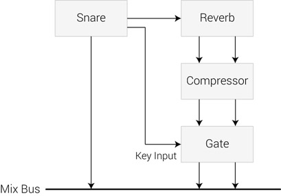
Figure 24.15 Gated snare setup. A schematic signal flow for an “improved” gated reverb.
If instead of decaying linearly the decay shape is altered so it sustains at maximum level (or falls slowly) and then decays abruptly, the reverb becomes more prominent. To achieve this, a compressor is inserted after the reverb. The compressor is set to flatten the decay so it hovers longer at higher amplitudes. But this will result in a reverb that might not drop below the gate’s threshold. Therefore, the original sound is sent to the gate’s key input. Figure 24.15 demonstrates such a setup.
There are endless numbers of productions in which gated reverb has been applied on snares and toms, but it can be applied to many other instruments, even those of a non-percussive nature. Shaping the reverb’s decay envelope can give the reverb more punch or more defined rhythmical characteristics (which must be observed while tweaking the gate). Gated reverbs are so popular that many digital reverb emulators include such a program. Still, better control is usually achieved by setting up the independent building blocks.
While gated reverbs are often used on drums, nonlinear reverbs in general can give the reverb more entity and a stronger rhythmic form.
![]()
Track 24.94: SnareTom Source
The source drum sequence before the addition of reverb.
Track 24.95: SnareTom Reverb Only
Both the snare and the toms are sent to the same reverb, which on this track is neither compressed nor gated.
Track 24.96: SnareTom Compressed Reverb
The reverb in this track has been compressed but not gated.
Track 24.97: SnareTom Compressed Gated Reverb
This is essentially the common gated reverb effect. The reverb is both compressed and gated.
Track 24.98: SnareTom Uncompressed Gated Reverb
Removing the compressor preceding the gate results in the effect heard on this track.
Plugins: Sonnox Oxford Reverb, Digidesign DigiRack Expander/Gate Dyn 3
Drums: Toontrack EZdrummer
Reverse reverbs and preverb
A reversed reverb does not really reverse any audio, but it does reverse the amplitude envelope of the reverb, so it starts quietly, grows gradually, and then cuts abruptly (Figure 24.16a). This effect gives a backward impression that can be used as a special effect.
A more common practice in mixing is called preverb. This is done by recording the reverb and then playing it backward so that it rises before the actual sound (Figure 24.16b). In order for this to work, the reverb has to be fed with a backward version of the original material. With tapes, this is easily done by reversing the reels, recording the reverb on to an available track and then reversing the reels again. In the digital domain, the original material has to be reversed, the reverb has to be bounced, and then both the original sound and the reverb have to be reversed again.

Figure 24.16 (a) A reversed reverb. (b) Preverb. The bold line denotes the direct sound.
![]()
Track 24.99: Reversed Reverb Mono
Both the dry voice and the reverb are panned hard-center in this track.
Track 24.100: Reversed Reverb Stereo
The voice is panned hard-left and the reverb to hard-right. This makes the reversed development of the reverb easier to discern.
Plugin: Logic EnVerb
As with the previous two tracks, the following two demonstrate preverb.
Track 24.101: Preverb Mono Track 24.102: Preverb Stereo
Track 24.103: Preverb Before Reversing
This is the voice and the reverb, before reversal.
Plugin: Universal Audio RealVerb Pro
Reverbs in practice
Reverb quantity and allocation
A common mixing discussion relates to the amount of reverbs one should use in a mix. To start the debate, one should imagine oneself in a standard professional studio back in 1971. Such a studio had mostly analog equipment, maybe up to three high-range dedicated reverb units, perhaps along with a couple of less expensive units and a few multi-effect units that had reverb programs as well. It would be fair to say that for most mixes in such a setup, the high-range units were allocated to ambiance and vocals, while other reverbs were allocated based on their quality and the importance of the instruments sent to them. Any mix that involved more than eight reverbs would be considered as reverb-happy, with many mixes completed with no more than five reverbs and some with as few as two. Previously, there was little choice other than to feed the same reverb unit with more than one track using an aux send. While there are mixes from that era that involve more than a dozen reverb emulators, it is worth remembering that many beloved mixes from the past were mixed with just a few reverb units. This practice still remains.
The inherent problem with hardware units is that they cannot be multiplied with a click of a mouse like plugins can. Even in 2001, many mixing engineers had to limit the number of reverb plugins due to processing power limitations, and reverbs had to be connected in parallel and in many cases were fed with a mix of many tracks using an aux send.
It is only in recent years that computers have become powerful enough to accommodate even 100 reverb plugins in a single mix. A different reverb plugin can be used as an insert on each individual track and one can also feed a single vocal track into five reverb plugins connected in series. Nowadays, for many of those who software-mix, having eight reverbs in a mix does not seem lavish at all.
If mixing engineers back in 1971 had had an array of 20 reverb units, they might have used them all. But two issues come to mind. The first is the fact that it is easier to grow a tree than a forest. Put another way, a mixing engineer might be tempted to use many reverb plugins while compromising on quality and giving less attention to each reverb. Selecting and configuring a reverb can be a truly time-consuming business, especially for the less experienced engineers who are not yet familiar with their tools. Second, the use of too many reverbs, especially if a different program is loaded onto each, can cause what is known as ambiance collision— a blend of too many spaces, which does not make any spatial sense. A certain objective when using reverbs is the creation of a firm, convincing ambiance even when an imaginary ambiance is involved. Although many reverbs can work together, a certain risk exists if insufficient attention is given to how they interact. Generally speaking, when using more than one ambiance reverb, softening the highs of the short reverbs can help conceal them and reduce collision.
While there is almost total agreement that expensive emulators are superior in producing a natural reverb, it is sometimes the cheapest and most basic emulators that can produce a distinctive effect. One advantage that comes with software plugins is that there is an ever-growing selection—some of today’s plugins offer unique controls and sound that might not be found in expensive emulators.
![]()
The dry signal used in the following samples.
Track 24.105: MultiAmb One Reverb
The woodblock, tambourine, and congas are all sent to the same reverb emulator.
Track 24.106: MultiAmb Three Reverbs
The three instruments are each sent to a different reverb emulator loaded with a different preset. We can still localize the instruments in the depth field, but the simulated space is less coherent than in the previous track.
Plugin: Universal Audio DreamVerb
Percussion: Toontrack EZdrummer
Aux send or insert?
Convention has it that reverbs are fed via auxiliary sends. The most obvious advantage in using a send is that we can send more than one signal to the reverb emulator, and therefore save processing power or share high-quality emulators. Connecting reverbs as a send on an analog desk requires just a few more easy steps compared with an insert connection. However, in the digital domain, the same task usually requires a little extra work, for example the creation of auxiliary tracks and bus routing. If many reverbs are used, but each is fed from one single track, the multitude of auxiliary tracks can clutter the mixer, and many buses are employed purely for routing purposes (rather than summing). Therefore, some argue that in specific situations, it is sensible to use an insert rather than a send, for instance when a reverb is added to a kick for two bars only, or when the reverb only adds a touch of early reflections that are meant to enrich a mono signal. One thing to remember is that when connecting as an insert, the reverb should output both the dry and wet signals; on both analog and DAW setups, changing the amount of reverb requires more effort than altering the send level, like when reverbs are connected as sends.
Another important point worth considering is that both in the analog and digital signal flows, the inserts are pre-fader. Thus, connecting reverbs as an insert forces a pre-fader feed that leaves all dry/wet adjustment to the reverb emulator. Accessing the emulator every time we want to change the dry/wet balance is somewhat less convenient compared with accessing the send controls.
In all but very specific situations, reverbs are added using sends.
Pre- or post-fader?
As just mentioned, reverbs connected as an insert are pre-fader (with rare exceptions). When connected as an aux send, we have a choice between either a pre- or post-fader send. A post-fader send is also post-cut. Similarly, a pre-fader send is also pre-cut.
The basic principle behind using post-fader send is that the level of the dry signal and the reverb level are linked—when the dry signal level increases, the reverb level increases as well. In practice, sometimes a fader adjustment might not lead to the desired reverb level change, and some additional adjustment to the reverb level will be needed. A post-fader send is necessary if any level or mute automation should take place—when we fade out or mute the dry signal, we want the reverb to fade out or mute as well.
Another point relates to the common use of destructive solos during mixdown. Say we have vocal and guitar both sent to an ambiance reverb. The reverb is solo safe to prevent it from being cut when other instruments are soloed. If the guitar send is pre-fader and the vocal is soloed, the guitar reverb will still be heard along with the vocal and its reverb. This can be highly annoying. Post-fader sends ensure that such situations do not occur.
Post-fader reverb send is most common in mixing, and is requisite if any level or mute automation is to take place on the source signal.
In some situations, we need to bounce the reverb separately from its dry signal. In many software applications, this can be achieved by soloing the reverb auxiliary track, but, as software solos are often destructive, this will cut the dry signal track as well. In order to still have the dry signal feeding the auxiliary bus, and consequently the reverb unit, a pre-fader send can be used. Another situation where a pre-fader send can be beneficial is when the original track is mixed at a very low level, and therefore the post-fader send will not provide enough level to produce an audible reverb.
Pre-compressor reverb send
Some interesting results can be achieved if the dry signal is compressed but the signal sent to the reverb emulator is taken before the compression takes place. In a performance with vibrant dynamics, increased expression is conveyed by louder phrases. Such a performance might be a problem in a mix and require compression. But, if sent to a reverb unit before being compressed, the dynamics of the performance will trigger more reverberation during the louder moments. This “manual automation” effect is most suitable on a performance with quick dynamic changes, such as some vocal performances.
While on an analog desk a copy of the uncompressed signal can always be taken from the multitrack return or a pre-processing insertion point, software users might scratch their heads wondering how this can be done—a software send (the reverb) is always post-insert (the compressor). Figure 24.17 illustrates how this can be done in Logic—the dry signal is sent to a bus, on which the reverb is inserted. Note that the vocal track output is not set to the main mix bus, but to another bus on which the compressor is inserted.
![]()
Track 24.107: Post-Comp Rev Send
The uncompressed vocal used in the following samples.
Track 24.108: Post-Comp Rev Send
The reverb send in this track succeeds the vocal compressor.
Track 24.109: Pre-Comp Rev Send
In this track, first the uncompressed vocal is sent to the reverb emulator, only then being compressed. Notice how the reverb gets louder in relation to the level of the uncompressed voice.

Figure 24.17 A pre-compressor reverb send in Logic.
How loud? How much?
Back in the 1980s, when the use of digital reverb units became widespread, much excitement surrounded this new tool and reverbs manifested in many mixes. As time went by, mixing engineers started to make more relaxed use of reverbs, and the general tendency today is that reverbs serve the mix rather than being a sound in their own right. In some of today’s mixes, a trained ear will be able to identify many more reverbs than initially seem present—reverbs nowadays tend to be more transparent and subtler.
This might go against the intuition of many novice mixing engineers, who, having introduced it, wish to hear the reverb in the mix. But the beauty of a reverb can persist even if it is not very obvious. One way to check the effectiveness of reverbs, even if hidden, is by muting them and seeing how they contribute to the mix. Yet, in specific situations, having a bold, well-defined reverb is our aim; solo saxophone in a mellow production could be one of these situations.
Tuning ambiance
The standard way to create ambiance involves sending various instruments to one or more ambiance reverbs. However, the resultant ambiance can suffer from various issues due to the frequency content of the various instruments sent to the reverb. Playing such a crucial part, the ambiance in a mix can be enhanced using a specific advanced technique. It involves sending a modified version of the instruments sent to the mix bus to the ambiance reverbs. On an audio sequencer, this can be achieved by duplicating a specific track and disabling its standard output routing to the main mix. Yet, this track is sent to the ambiance reverb instead of the original. We can then process (mainly equalize) the ghost track in different ways, so as to tune it to the ambiance created by the reverb it is sent to.
Delay and reverb coupling
A very common mixing technique involves a blend between a delay and a reverb. Most often, this technique is used on vocals, but it can be applied to other instruments just as well. Blending a delay with a reverb is known to result in a more impressive effect than using one or the other. One way to look at it is as if the delay enhances the reverb. Multitap delays with two active taps (each panned to a different side of the panorama) are highly suitable for this task. Most often, the delay and the reverb are connected in parallel (i.e., neither feeds the other). On an audio sequencer, this can be achieved by sending a track to a bus, then feeding the bus into two different aux tracks—on one a reverb is loaded, on the other a delay. It also pays to try to connect a delay before a reverb—such an arrangement can also produce an appealing effect.
![]()
Track 24.110: Vocal Reverb No Delay
This track involves a reverb, but no delay.
Track 24.111: Vocal Reverb With Delay
The delay in this track is added in parallel to the reverb. Notice how, compared to the previous track, the effect here sounds slightly livelier and richer.
Plugins: Audio Ease Altiverb, PSP 82
Reverb coupling
Sometimes we combine two reverbs in order to achieve a specific task. However, this has to be done with caution or some problems might arise. Coupled reverb is the term used to describe a “reverb of a reverb.” In real life, such a phenomenon can occur when a reverb from one space travels to an adjacent space that adds its own reverb. Coupled reverbs are mainly a concern for natural reverb simulations—they place a space within a space, they increase the reverb time, and they introduce reverbs that can have broken decay slopes. In mixing, coupled reverbs can be introduced with the addition of a reverb to a recording that already contains a reverb or when connecting two reverb emulators in series.
Recordings that include a reverb, unless initially intended, can sometimes create great difficulties for the mixing engineer, and in extreme situations can be unusable. Such recordings are sometimes done by inexperienced recording engineers who may choose to record a guitar amp or an electronic keyboard with their internal (sometimes monophonic) cheap reverb effect. Sometimes a recorded reverb is simply the result of a very reverberant recording environment. One way or another, such reverbs are then imprinted into the recording, often sound cheap, and leave the mixing engineer between a rock and a hard place. It is worth remembering that reverbs often become louder after being compressed. Compressing a vocal recording that contains reverb can result in solid vocal levels but fluctuating reverb. While it is only possible to achieve a completely reverb-free recording in an anechoic chamber, recording engineers can achieve a direct-to-reverb ratio that will present no limitations during mixdown.
With the exception of a recording that was intended to capture ambiance, a reverb on a recording is like oil on water—they are likely to not mix well.
Nonetheless, a combination of two reverb emulators during mixdown can be useful. A valid practice is to send the same signal to two reverb emulators that are connected in parallel. This creates a composed reverb that can have a richer texture. Another possible experiment that can yield an interesting effect is using two mono reverbs and panning each to an opposite extreme.

Figure 24.18 Reverb coupling. (a) Parallel reverb setup where each emulator produces a different reverb component. (b) Serial reverb setup where the early reflection from the first emulator feeds the second emulator, which only generates reverberation.
Yet another trick relates to the way emulators work—many of them have separate engines for the early and late reflections. Some emulators feed the early reflections into the late reflection engine, while others have complete separation between the two. Often we can choose the balance between the early and late reflections or simply switch off one engine or the other. This yields some interesting possibilities where we can combine two emulators, each producing either the early or later reflections. If we have two emulators and one is better at producing early reflections while the other is better at producing reverberation, we can mute the weak engine in each emulator to achieve a reverb that has the best of both worlds. This can work exceptionally well when a convolution reverb is the generator of the early reflections. Convolution reverbs tend to produce a highly believable early reflection pattern, but might be very CPU-consuming if the long reverberation is produced as well. By assigning the convolution reverb with the task of producing the early reflections only, and assigning the less critical task of late reflections to an algorithmic reverb, we can save CPU power, yet end up with more convincing results. The emulators can be connected either in parallel or in series, depending on whether we want to feed the early reflections into the late ones (Figure 24.18).