16
Introduction to dynamic range processors
Chapters 17–21 deal with compressors, limiters, gates, expanders, and duckers. All fall into a group called dynamic range processors. The similarities between them are worth discussing as a background to the succeeding chapters.
Dynamic range
Dynamic range is defined as the difference between the softest and loudest sounds a system can accommodate. Our auditory system, digital systems (such as an audio sequencer), and analog systems (such as a loudspeaker) all have their dynamic range. Absolute level measurements are expressed using various dB scales—dBSPL, dBu, dBFS, etc. Dynamic range, like any difference between two level measurements, is expressed in plain dB. The table below shows the dynamic range of various systems.
| System | Approximate dynamic range (dB) |
|
|
|
| Software mixer (25 bits) | 150 |
| Best A/D converters available | 122 |
| Human hearing | 120 |
| Dynaudio Air 25 Active Monitors | 113 |
| Neumann U87 Condenser Microphone | 110 |
| CD, or 16-bit integer audio file | 96 |
| Tape with noise reduction | 75 |
| FM radio | 65 |
| Vinyl | 60 |
Say the quietest moment of an orchestral piece involves a gentle finger tap on the timpani, which generates 10 dBSPL. Then at the loudest moment the orchestra emits 100 dBSPL. That is a musical piece with 90 dB of dynamic range. A U87 microphone placed in the venue would theoretically be able to capture the full dynamic range of the performance, including both the quietest and the loudest moments (although during the quietest moments the microphone noise might become apparent, and during the climax the microphone might distort). All but the cheapest A/D converters can accommodate 90 dB of dynamic range, so when the microphone signal is converted to digital and recorded onto a computer the dynamic range of the performance is retained. The full dynamic range will also remain if the performance is saved onto a 16-bit integer file, or played through good studio monitors.
However, we will encounter a problem cutting this performance on vinyl—we have to fit 90 dB of dynamic range into media that can only accommodate 60 dB. There are a few things we can do. We can just trim the top 30 dB, so every time the orchestra becomes loud it is muted—an idea so senseless that no processor is designed to operate this way. We can just trim the bottom 30 dB of the performance, so every time the orchestra gets really quiet there will be no sound. Also not the wisest idea, although we do something similar every time we bounce from our audio sequencer (25 bits) into a 16-bit file—we trim the bottom 9 bits (reducing from 144 to 96 dB).
![]()
How much is 60 dB? Readers are welcome to experiment: use pink noise from a signal generator, and bring it down by 60 dB using a fader. Chances are that at –60 dB you would not hear it. Now boost your monitor level slightly in order to hear the quiet noise, and then slowly bring the fader back up to 0 dB. Chances are you will find the noise fairly loud, and you might not even fancy bringing the fader all the way up; 60 dB is regarded in acoustics as the difference between the loud and the inaudible. We will discuss this further in Chapter 24 when we look at reverbs. The 60 dB experiment might be disappointing for some—you might wonder where half of our 120 dB hearing ability went. The auditory 120 dB was devised from what was thought to be the quietest level we can hear—0 dBSPL—and the threshold of pain, which is around 120 dBSPL. In practice, most domestic rooms have ambiance noise at roughly 30 dBSPL; 120 dBSPL is the level you’ll be exposed to when standing a meter from the speaker in an extremely loud rock concert or a dance club. Under such circumstances, you might not be able to hear someone shouting next to you. A shouting voice is roughly 80 dBSPL. We perceive 90 dBSPL as twice as loud, which is already considered very loud. If there is such a thing as the dynamic range of everyday life, it is somewhere between 30 and 70 dBSPL—40 dB of dynamic range. Still, a studio control room may feature a dynamic range from 20 to 110 dBSPL.
Having said that, we might still want our vinyl to retain both the loudest and softest moments of our orchestral performance, and trimming would not let us do so. What we can do is compress the dynamic range. We can make loud levels quieter—known as downward compression; or we can make soft levels louder—upward compression. By way of analogy, it is like squeezing a foam earplug before fitting it into our ear—all the material is still there, but compressed into smaller dimensions.
Say we have the opposite problem: we have an old vinyl that we want to transfer onto a 16-bit audio file. We might want to convert 60 dB of dynamic range into 96 dB. A process called expansion enables this. We can make quiet sounds even quieter—downward expansion; or we can make loud sounds even louder—upward expansion. This is similar to what happens when we take the earplug out—it returns to its original size.
![]()
By and large, downward compression is the most frequent type of compression in mixing, and so the word “downward” is omitted by convention—a compressor denotes a downward compressor. It is the same with expansion—downward expansion is more common, thus “downward” is omitted. This book follows these conventions.
Now how does this relate to mixing? Well, very little … but at the same time, quite a lot. It is the mastering engineer’s responsibility to fit the dynamic range of a mix onto different kinds of media (and they do compress vinyl cuts). Nowadays, with the decreasing popularity of tape machines, we hardly change between one system and another—during mixdown, we care little about the overall dynamic range of our mix. However, very often while we mix we want to make loud or quiet sounds louder or quieter. It is rarely the overall dynamic range we have in mind—what we really want to control is the dynamics of instruments.
Dynamics
The term dynamics in mixing is equivalent to the musical term—variations in level. Flat dynamics mean very little or next to no variations in level; vibrant dynamics mean noticeable variations; wild dynamics mean excessive fluctuations that are somewhat disturbing.
We distinguish between macrodynamics and microdynamics. In this book, macrodynamics are regarded as variations in level for events longer than a single note. We talk about macrodynamics in relation to the changing level between the verse and the chorus, or the level variations between snare hits, bass notes, or vocal phrases.
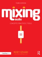
Microdynamics are related to level variations that happen within each note being played due to the nature of an instrument; for example, the attack and decay of a snare hit. We associate microdynamics with the dynamic envelope of sounds, which entail level variations that happen within each note (or hit) being played. The dynamic envelope constitutes the second half of an instrument’s timbre (the first half being the spectral content). We can associate different envelopes with different instruments, as Figure 16.1 demonstrates. It is worth knowing that most instruments have some initial transient or level burst as part of their dynamic envelope. Very often, we employ dynamic range processors to control the microdynamics in these envelopes or reshape them to alter the instrument’s timbre.
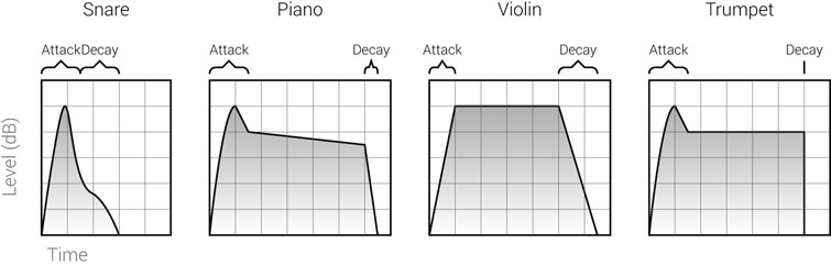
Figure 16.1 The typical dynamic envelope of various instruments. A snare has a quick attack caused by the stick hit; the majority of the impact happens during the attack stage, and there is some decay due to resonance. A piano also has an attack bump due to the hammer hitting the string; as long as the key is pressed, the sustained sound drops slowly in level; after the key is released, there is still a short decay period before the damping mechanism reaches full effect. The violin dynamic envelope in this illustration involves legato playing with gradual bowing force during the initial attack stage; the level is then kept at a consistent sustain level, and, as the bow is lifted, string resonance results in slow decay. In the case of a trumpet note, the initial attack is caused by the tongue movement; consistent airflow results in a consistent sustain stage, and as the airflow stops the sound drops abruptly.
![]()
It is worth noting the terminology used in Figure 16.1 and throughout this book. The attack is the initial level buildup and includes the fall to sustain level. Decay is used to describe the closing level descent. This is different from the terminology used for a synthesizer’s ADSR (attack, decay, sustain, release) envelope.
Dynamic range processors in a nutshell
Transfer characteristics
Say we regard an electrical wire as a processor, and its ends as the input and output. Practically speaking, signals entering the wire pass through unaffected. For any given input level, we get the same output level. We can say that the level ratio between the input and output is 1:1. Such a ratio is known as unity gain. We can draw a graph that shows the relationship between the input and output levels. Such a graph is called a transfer characteristics graph, or input–output graph, and is said to show the transfer function of a processor. It shows the input level on the horizontal axis and the output level on the vertical axis. The scale is given in decibels; 0 dB denotes the reference level of the system— the highest possible level of a digital system (which cannot be exceeded) or the standard operating level of an analog system (which can be exceeded). Figure 16.2 shows the transfer function of an electrical wire.
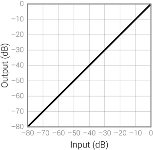
Figure 16.2 The transfer function of an electrical wire. There is no change in level between the input and the output—in other words, unity gain throughout.
As opposed to wires, dynamic range processors do alter the level of signals passing through them—the input and output levels might be different. We already know that a compressor reduces dynamic range, so we can expect input levels to be brought down. Figure 16.3 shows the transfer function of a compressor. We can see that the output’s dynamic range is half that of the input.
If all dynamic range processors behaved like the compressor in Figure 16.3, they would all be rather limited (in fact, the earliest dynamic range processors were limited very much in this way). Treating all levels uniformly is rarely what we want, even in cases where it is the whole mix we are treating. Most of the time, we only want to treat a specific level range—commonly either the loud or quiet signals. To enable us to treat selectively, all dynamic range processors allow us to limit treated levels and untreated levels using a parameter called threshold.
Figure 16.3 The transfer function of a compressor. The output dynamic range is half the input dynamic range.
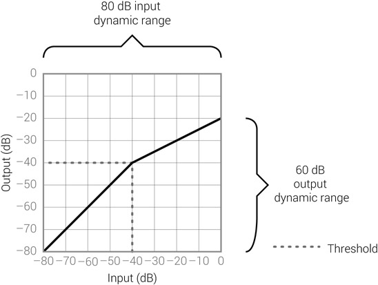
Figure 16.4 A compressor with threshold. The threshold is set to –40 dB. Levels below the threshold are not treated, and the input to output ratio is 1:1. Above the threshold, input signals are brought down in level. In this specific illustration, the input-to-output ratio above the threshold is 2:1.
The threshold divides the full input level range into two sections. Depending on the processor, the treated level range might be above or below the threshold. Figure 16.4shows a compressor with the threshold set at –40 dB. Being a downward compressor, loud levels are made softer, but only above the threshold—levels below the threshold are unaffected. Note that the output dynamic range has been reduced. It is also worth noting that the input-to-output ratio above the threshold is 2:1, resulting in the top 40 dB of input range (–40 to 0 dB) turning into 20 dB at the output (–40 to –20 dB). We will discuss ratios in greater detail in the following chapters.
The function of different processors
Figure 16.5 shows the transfer function of various dynamic range processors, and how levels are altered between the input and output. Here is a quick summary of what each of these processors does:
- Compressor—reduces the level of signals above the threshold, making loud sounds quieter.
- Limiter—ensures that no signal exceeds the threshold by reducing any signals above the threshold down to the threshold level.
- Upward compressor—boosts the level of signals below the threshold, making quiet sounds louder.
- Expander—reduces the level of signals below the threshold, making quiet sounds quieter.
- Upward expander—boosts the level of signals above the threshold, making loud sounds even louder.
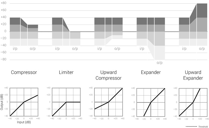
Figure 16.5 Sample transfer functions of compressors, limiters, and expanders, and their effect on input signals. The bottom graphs show the transfer function of each processor, all with threshold set to 0 dB. The top row illustrates the relationship between the input and output levels.
All the processors above apply some ratio while transforming levels, making the level change dependent on the input level. For example, the compressor above has a 2:1 ratio above the threshold; +40 dB at the input is reduced to +20 dB (20 dB level change), while +20 dB is reduced to +10 dB (10 dB level change). The ratio of reduction is identical, but the level change is different.
Gates work on a slightly different principle—all signals below the threshold are reduced by a fixed amount known as range. With large range settings (say, –80 dB), signals below the threshold become inaudible, A ducker also reduces the signal level by a set range, but only does so for signals above the threshold. Figure 16.6 shows the function of a gate and a ducker, which can be summarized as follows:
- Gate—attenuates all signals below the threshold by a fixed amount known as range. Drastic attenuation makes everything below the threshold inaudible.
- Ducker—attenuates all signals above the threshold by a fixed amount—also known as range.
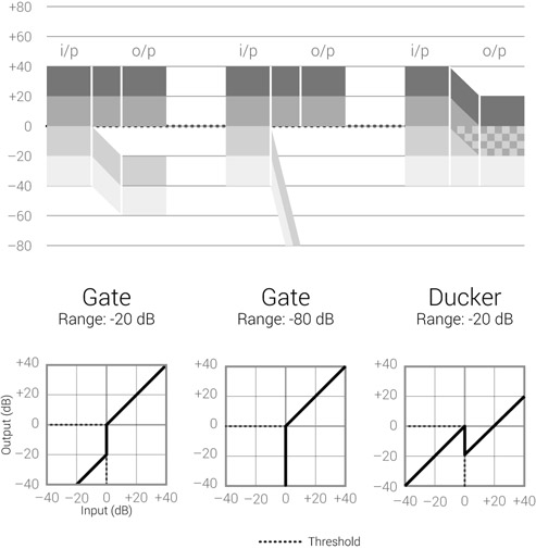
Figure 16.6 The transfer function of a gate with different range settings and a ducker. With small range settings, the gate simply attenuates everything below the threshold. With large range settings, the gate is said to mute signals below the threshold. A ducker attenuates signals above the threshold by a set range.
Pumping and breathing
Dynamic range processors can produce two artifacts known as pumping and breathing. Pumping is caused by quick, noticeable variations of level. We usually associate pumping with loud level variations, such as those that can be the outcome of heavy compression or limiting. Breathing is the audible effect caused by varying noise (or hiss) levels. Often it is the quiet level variations that produce such artifacts, mostly due to the operation of gates or expanders.
![]()
Tracks 16.2 and 16.3 demonstrate pumping. The threshold on the compressor is set to –45 dB, the attack is set to slow, and the ratio is set to 60:1. In all of these tracks, the kick triggers the heaviest compression. It is worth noting the click on the very first kick, which is caused by the initial, drastic gain reduction.
Track 16.1: Original (No Pumping)
Track 16.2: Pumping (Fast Release)
The quick gain reduction and recovery is evident here. For example, the level of the hats fluctuates severely.
Track 16.3: Pumping (Medium Release)
The medium release causes slower gain recovery, which means levels fluctuate less. Although not as wild as in the previous track, the level changes are still highly noticeable.
Track 16.4: Pumping (Slow Release)
The slow release means that the gain hardly recovers before the next kick hits. The resultant effect cannot really be considered as pumping, since the gain fluctuations are too slow. However, it is hard to overlook how such slow recovery adds some dynamic movement to the loop.
Track 16.5: Breathing
The fluctuating noise level is associated with the term “breathing.” The vocal and the underlaid noise pass through a gate/compressor—both respond to the vocal. The gate causes the noise to come and go, while the varying amount of gain reduction on the compressor results in fluctuating noise level.
Plugin: Universal Audio GateComp