
17
Compressors
Perhaps the most misused and overused tool in mixing is the compressor—which is especially worrying considering how predominant compressors are in contemporary mixes. It is no secret that compressors can make sounds louder, bigger, punchier, richer, or more powerful. Neither is it a secret that, since compressors were introduced per channel on analog consoles, the amount of compression in mixes has grown progressively and significantly—from transparent compression to evident compression, to heavy compression, to hypercompression, to ultracompression, so that by the start of the new millennium compression had been applied in so many mixes to such massive degrees that some people find it absurd:
- —Are these VU meters broken?
- —No.
- —So why aren’t they moving?
- —Ah! It’s probably my bus compression. Sounds like the radio, doesn’t it?
If used incorrectly or superfluously, compressors suppress dynamics. Dynamics are a crucial aspect of a musical piece and a key messenger of musical expression. How impossible would our lives be if we could not alter the loudness of our voices? How boring would our singing be? A drummer would sound like a toy drum machine, and every brass instrument would resemble a car horn. If anything is to blame for the lifeless dynamics in contemporary music, it is the ultracompression trend.
A significant milestone in the story of compression was the release of Metallica’s Death Magnetic in 2008. An album whose sound quality was so badly compromised by ultracompression—the hallmark of the infamous loudness war—that it didn’t take a pair of trained ears to notice: the public complained. Subsequently, the term loudness war erupted from its oblivious boundary within the audio and music industries into the general public with help from national newspapers and social media. All because of one album, a decade or so too late in the view of many audio professionals.
Luckily, in recent years, more and more mixing and mastering engineers have left the ultracompression club and reverted back to more sensible compression. That’s not to suggest that compressors should not be used, or used subtly. Many mixes still benefit from a hard-working compressor on many tracks. The real secret is to retain musical dynamics. We also have to distinguish the tightly controlled dynamics of pop music and the loss of dynamics caused by ultracompression. Some mixes present tightly controlled dynamics, yet instruments sound alive. Ultracompression is not a requisite for commercial success; if anything, it is a threat.
One specific problem novice engineers have is that they do not know how the dynamics of a mix should sound. All they have for comparison is the dynamics of a mastered mix or, worst still, the dynamics of a mastered mix played through the radio. The latter can often sound squashed to death compared with a premastered mix. By trying to imitate the sound of a mastered album or the radio, the novice can easily limit the quality of the final master. Reviving a lifeless mix during mastering is hard; but if a mix has vibrant dynamics, mastering engineers can treat it as much as they want or are asked to.
One must pay attention to musical dynamics when compressing.
People often underestimate how hard compressors are to master. Making a beat punchy is not as easy as simply compressing it. There are numerous controls we can tweak and most of them are correlated. In order to obtain excellent results from a compressor, we must first understand how it works, the function of each control, and how these affect the dynamic behavior of each treated instrument. A compressor is such a powerful and versatile tool that some of its many applications are polar in nature (e.g., softening transients or emphasizing transients). Perhaps, after reading this chapter, those who used compressors in the past will feel that they have been flying a spaceship when they thought they were driving a car. It is a long chapter, but the knowledge provided can make the difference between the flourish techniques of the seasoned pro and the random trials of the novice. The consequences for the mix can be profound.
The course of history
One problem in early radio transmissions was that, if program levels exceeded a certain threshold, the transmitter would overload and blow—never a good thing, particularly during the climax of a thrilling sports broadcast. Radio engineers had to observe levels meticulously and ride the gain of live broadcasts so that levels did not exceed the permitted threshold (Figure 17.1). While these engineers did their best, only a fortune teller could predict sudden level changes, and it was safe to assume that no fortune teller would apply for the job. Even if they did, there is a limit to just how quickly one can respond to sounds or physically move a fader—sudden level changes would still be an issue. While peak control was aimed at protecting the transmitter, gain-riding was also performed in order to balance the level of the program, levelling the different songs and the presenter’s voice.
By the 1920s, people such as James F. Lawrence Jr. (who later designed the famous LA-2A) already had ideas about building a device that would automate the gain-riding process. The concept was to feed a copy of the input signal to a side-chain, which, based on the incoming level, would determine the required amount of gain reduction. The side-chain was connected to a gain stage, which applied the actual gain reduction on the signal (Figure 17.2). The name given to these early devices was leveling amplifier (suggesting more of a balancing function) or limiter (suggesting more of a peak control function). However, early models had very slow response to sudden level changes, and thus they did not really limit the level of the signal—they behaved very much like today’s compressors. With advances in technology, true limiting was eventually possible, and the distinction between compressors and limiters had been made.
Studio engineers quickly borrowed compressors for their recording studios as, just like radio engineers, they had to gain-ride live performances. At the time, it was necessary to contain peaks so that when music was cut on the fly to disc it would not distort. Later, it was utilized to protect tapes from saturating, and later still to protect digital systems from clipping. Compressors were also employed to even out the dynamics of a performance; for example, when vocals change from soft to loud. By the 1960s, units such as the Urei 1176 LN, Fairchild 670, and LA-2A were already a common sight in control rooms.

Figure 17.1 Manual gain-riding. The engineer gain-rides levels with relation to the speaker output. In this illustration, a VCA fader is employed.

Figure 17.2 (a) A feedback-type compressor. The input into the side-chain is taken past the gain stage, which resembles the way manual gain-riding works. Early compressors benefited from this design as the side-chain could rectify possible inaccuracies of the gain stage (for example, when it did not apply the required amount of gain reduction). However, this design had more than a few limitations; for instance, it did not allow a look-ahead function. (b) A feed-forward type compressor has the input into the side-chain taken before the gain stage. As most modern compressors are based on this design, it will be discussed in the rest of this chapter.
Compressors alter both the dynamic envelope of the source material and, like any other nonlinear device, add some distortion—together we get the distinctive effect of compression. The original intention of compressors was to alter the dynamic range while leaving as little audible effect as possible. However, it soon became apparent that the effect of compression, like that caused by an overloaded tape, can be quite appealing. One sonic pioneer who understood this was Joe Meek, who, instead of concealing the effect of compressors, used it as part of his distinctive sound. Among his many highly acclaimed recordings was the first British single ever to top the U.S. Billboard chart— “Telstar” by The Tornados (1962). Nowadays, the effect of compression can be heard in nearly every mix.
Sometimes we want the compressor to be transparent. Sometimes we use it for its distinctive effect.
When it comes to the use of a compressor as a level balancer, the end to this brief history is somewhat interesting. The compression effect becomes more evident with heavier compression. If a vocal performance changes from crooning to shouting, the effect will be more noticeable on the shouting passage, being subject to more compression. While after compression the performance might appear to be consistent in level, the shouting passage could have a distinct compression effect that will be missing from the crooning passage. To combat situations such as this, manual gain-riding still takes place before compression (despite the latter being invented to replace the former).
The sound of compressors
No two compressor models sound alike, certainly no two analog compressors. Some can work better for drums and some can work better on vocals; some add warmth, some an extra punch; some can be transparent while others produce a very obvious effect. Each compressor has a character, and in order to have a character something must be different from its counterparts.
We can generalize what we want from a precise compressor; here are just a few points:
- We want compression to start at a consistent point with relation to the threshold.
- We want the gain stage to act uniformly on all signal levels and with consistent response times.
- We want accurate performance from the ratio function.

Figure 17.3 Top: the TL Audio VP-5051. Middle: the Urei 1178 (the stereo version of the 1176). Bottom: Drawmer DL241. The three have distinctively different sounds. Source: Courtesy of SAE, London.

Figure 17.4 A compressor plugin: the Digidesign DigiRack Compressor/Limiter Dyn 3.
- We want to have the ability to dial attack and release times of our choice, even if these are very short.
- We want the attack and release envelopes to be consistent and accurate.
In practice, there is little challenge building a precise digital compressor. A quick online search will quickly yield a free algorithm for exactly such a compressor, but it won’t have character. Analog designs have a character due to their lack of precision, and each compressor is inaccurate in its own unique way. How the ratio behaves or the nature of the attack and release functions defines much of the compressor sound. It is mostly these aspects that earned vintage models much of their glory. In order to introduce some character into digital compressors, designers have to choose where and how to introduce deviations from the precise design.
Principle of operation and core controls
The explanation of how compressors work is often oversimplified and inaccurate. To really understand how this popular tool works, it is imperative to look at its internal building blocks—consisting of a few simple stages. Figure 17.5 focuses on the main stages and the controls linked to each. The illustration is based on the modern VCA analog design— pretty much the blueprint for most modern compressors, including digital ones.
Gain
The gain stage is responsible for attenuating (and in some cases also boosting) the input signal by a set number of dBs (which is determined by the side-chain). The gain stage in Figure 17.5 is based on a VCA, but other types of gain stages may be used. It pays to learn the differences between them, if only because many of today’s digital compressors try to imitate the sound of old analog ones:
- Vari-mu—the earliest compressor designs were based on variable-mu tubes (valves); essentially, variable gain amplifiers. Vari-mu designs have no ratio control; they apply incremental amount of gain reduction with relation to input levels (a behavior similar to soft-knee, which is explained later). But this only happens up to a point, when the compressor returns to linearity. This characteristic works well for percussive instruments as loud transients are not clamped down. Vari-mu designs have faster attack and release times than optical designs, but they are not as fast as VCA designs or FET.

Figure 17.5 Inside a compressor. The vertical chain shows the main stages within the side-chain, and the controls link to each stage. The nature of the signal between one stage and another is shown to the left of the chain, along with a sample graph that is based on the settings shown under each control name.
- FET—as small transistors started replacing the large tubes, later compressor designs were based on field effect transistors (FETs). They offered considerably faster attack and release times than vari-mu and incorporated a new feature—ratio. Just like vari-mu designs, the compression ratio tends to return to linearity with a very loud input signal.
- Opto—the side-chain of an optical compressor controls the brightness of a bulb or LED. On the gain stage, there is a photo-resistive material, which affects the amount of applied gain. Much like our pupils takes a bit of time to contract and dilate in response to changing light intensity, photo-resistive material has slow response compared with musical dynamics; thus, optical compressors exhibit the slowest response times of all compressors. Moreover, their attack and release curves are less than precise (especially with older designs), giving these compressors a very unique character. Optical designs are known to produce a very noticeable effect, which many consider appealing.
- VCA—of all their analog equivalents, solid-state voltage-controlled amplifiers (VCAs) provide the most precise and controllable gain manipulation. Their native accuracy broadened the possibilities compressor designers had, and made VCAs the favorite in most modern designs.
- Digital—digital compressors work using a set of mathematical operations. When it comes to precision, a digital compressor can be as precise as it gets. Their response time can be instant, which means no constraints on attack and release times. Digital compressors can also offer perfectly precise ratio, attack, and release curves.
Level detection and peak vs. RMS
As the signal enters the side-chain, it first encounters the level stage. This is where its bipolar amplitude (Figure 17.5a) is converted into a unipolar representation of level (Figure 17.5b). At this point, the level of the signal is determined by its peak value. Instead of peak-sensing, it might be in our interest to have RMS-sensing, so the compressor responds to the loudness of incoming signals rather than to their peaks (vocals are often better compressed that way). An RMS function (or other averaging function) might take effect at this stage. By way of analogy, it is as if we have replaced a peak meter within the level stage with a VU meter.
A compressor might support peak-sensing only or RMS-sensing only, or offer a switch to toggle between the two. Some compressors also allow us to dial a setting between the two. If no selection is given, the compressor is likely to be an RMS one.
Threshold
The threshold is the level above which gain reduction starts. Any signal exceeding the threshold is known as an overshooting signal and would normally be reduced in level. The more a signal overshoots, the more gain reduction is applied. Signals below the threshold are generally unaffected (we will look at two exceptions to this later). The threshold is most often calibrated in dB.
A threshold function on a compressor comes in two forms: a variable threshold or a fixed threshold. A compressor with variable threshold provides a dedicated control with which the threshold level is set. A compressor with fixed threshold (Figure 17.7) has an input gain control instead—the more we boost the input signal, the more it will overshoot the fixed threshold. This is similar to the way compression is achieved when overloading tapes. To compensate for the input gain boost, an output gain control is also provided. One advantage of the fixed threshold design (with analog units, anyway) is that the noise introduced by the gain stage is often attenuated by the output gain. On variable threshold designs, the same noise is usually boosted by the output (or makeup) gain in order to compensate for the applied gain reduction.
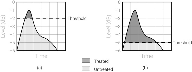
Figure 17.6 Threshold setting. (a) Higher threshold means that a smaller portion of the signal is treated. (b) Lower threshold results in a larger portion of the signal being treated.
![]()
Track 17.1: Dropping Threshold
This track involves a continuously dropping threshold, from 0 dB down to –60 dB at a rate of –7.5 dB per bar. The compressor is configured to bring down signals above the threshold as quickly as possible (fastest attack: 10 µs) and as much as possible (highest ratio: 100:1). Therefore, the lower the threshold, the larger the portion of the signal being brought down in level, resulting in a gradual decrease in overall level.
Track 17.2: Dropping Threshold Compensated
This track is similar to the previous one, except after compression has been applied the track level is gradually boosted to compensate for the loss of level caused by the compressor. This reveals a better increasing compression effect over time.
Plugin: Digidesign DigiRack Compressor/Limiter Dyn 3
Drums: Toontrack EZdrummer

Figure 17.7 The Universal Audio 1176SE. This plugin for the UAD platform emulates the legendary Urei 1176LN. It has fixed threshold and the degree of compression is partly determined by the input gain amount.
As can be seen in Figure 17.5c, the threshold stage is fed with the level of the side-chain signal. The output of this stage is the overshoot amount, which indicates by how much an overshooting signal is above the threshold. For example, if the threshold is set to 2 dB and the signal level is 6 dB, the overshoot amount is 4 dB. If the signal level is below the threshold, the overshoot amount is 0 dB.
Ratio
Ratio can be compared with gravitational force, which determines the extent to which objects are pulled toward the ground. There is less gravity on the moon, so astronauts can jump higher. Ratio determines the extent to which overshooting signals are reduced toward the threshold. The lower the ratio, the easier it is for signals to jump above the threshold. Figure 17.8 shows the effect of different ratios on an input signal.
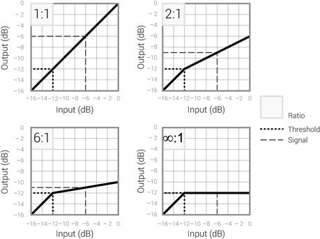
Figure 17.8 The effect of different ratios on the level envelope of a waveform.

Figure 17.9 Different ratios on transfer characteristics graphs. In all these graphs, the threshold is set to –12 dB and the input signal is –6 dB (6 dB above the threshold). With a 1:1 ratio, the output signal leaves the compressor at the same level of –6 dB (6 dB above the threshold); with a 2:1 ratio, the signal leaves at –9 dB (3 dB above the threshold); with a 6:1 ratio, the signal leaves at –11 dB (1 dB above the threshold); and with ∞:l, the signal leaves at the same level as the threshold.
Newtonian physics aside, once the signal overshoots the threshold, the ratio control determines the ratio between input and output level changes (as the input-output notation suggests). For example, with a 2:1 ratio, an increase of 2 dB above the threshold for input signals will result in an increase of 1 dB above the threshold for output signals. The ratio determines how overshooting signals are scaled down. A 1:1 ratio (unity gain) signifies that no scaling takes place—a signal that overshoots by 6 dB will leave the compressor 6 dB above the threshold. A 2:1 ratio means that a signal overshooting by 6 dB is scaled down to half of its overshoot amount and leaves the compressor at 3 dB above the threshold. A 6:1 ratio means that a signal overshooting by 6 dB is scaled down to a sixth and leaves the compressor at 1 dB above the threshold. The highest possible ratio is ∞:1 (infinity to one), which results in any overshooting signal being trimmed to the threshold level. Often, a ratio of ∞:1 is achieved by using an extremely high ratio such as 1,000:1. Figure 17.9 illustrates these four scenarios.
![]()
Track 17.3: Raising Ratio
This track involves a threshold at –40 dB and a continuously rising ratio from 1:1 up to 64:1. The ratio doubles per bar, starting with 1:1 at the beginning of the first bar, 2:1 at the beginning of the second bar, 4:1 at the beginning of the third bar, and so on. The higher the ratio, the harder overshooting signals are reduced toward the threshold, resulting in a gradual decrease in the overall level.
Track 17.4: Raising Ratio Compensated
This track is identical to the previous one, only that the loss of level caused by the compressor is compensated using a gradual gain boost. Here again, the increased compression effect over time is easily discerned.
Plugin: Digidesign DigiRack Compressor/Limiter Dyn 3
Drums: Toontrack EZdrummer
One characteristic of vintage compressors, notably vari-mu and FET designs, is that the ratio curve maintains its intended shape, but morphs back to unity gain with loud signals. This type of ratio curve tends to complement transients, as the very loud peaks are not tamed—compression is applied, but less dynamics are lost. Drum heaven. Many digital compressors imitate such a characteristic behavior by employing similar ratio curves. The McDSP CB1 in Figure 17.10 is one of them.
The ratio is achieved within a compressor by the scale stage (Figure 17.5). The scale stage is the operational heart of the compression process—this is where the overshoot amount is converted into the provisional gain reduction. The output of the scale stage is nearly fit to feed the gain stage. The ratio essentially determines the percentage by which the overshoot amount is reduced to 0 dB. A 1:1 ratio means that the overshoot amount is fully reduced to 0 dB, which means that no gain reduction takes place. With a 2:1 ratio, the overshoot amount is reduced by half. For example, 4 dB of overshoot becomes 2 dB.
Attack and release
Modern compressors can respond to sudden level changes instantly, but such quick response is not always sought. For example, in order to retain some of the instrument’s natural attack, we often want to let some of the initial level burst through the compressor unaffected (or lightly affected). In order to do so, we need to be able to slow down the compressor response times. Similarly, if a healthy amount of gain reduction drops too fast, the gain recovers too quickly, which may result in pumping. To prevent this, we need a way of controlling the rate at which gain reduction drops.
The attack and release are also known as time constants or response times. The attack determines how quickly gain reduction rises, while release determines how quickly gain reduction falls. Essentially, a longer setting on either will simply slow down the rate at which gain reduction increases (attack) or decreases (release). For example, in Figure 17.5d, the gain reduction rises instantly from 0 to 2 dB and then falls back instantly to 0 dB. Having 1 ms of both attack and release means, in this case at least, that it takes 1 ms for the gain reduction to rise and fall (Figure 17.5e).
Both the attack and release times are typically set in milliseconds. Attack times usually range between 0.010 ms (10 µs) and 250 ms. Release times are often within the 5–3,000 ms (3 seconds) range. It is important to understand that both times determine how quickly the gain reduction can change, and not the time it takes it to change. In practice, both define how long it takes the gain reduction to change by a set number of dB. For example, 1 second of release time might denote that it takes the gain reduction 1 second to drop by 10 dB. Accordingly, it would take it half a second to drop by 5 dB. This behavior can be compared with the ballistics of a VU meter. A quick peak drop would appear gradual on a VU meter. When peaks drop slowly, the VU reading will be very similar to that of a peak meter. The attack and release have a very similar effect on gain reduction.

Figure 17.10 The McDSP CB1 plugin. The input-output plot shows that compression starts around the threshold and then develops into heavy limiting. However, around –12 dB, the ratio curve changes course and starts reverting to unity gain. Ratio slopes of this nature, which deviate from the textbook-perfect shape, can provide a characteristic sound that is usually a trait of vintage analog designs.
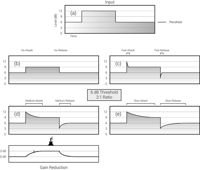
Figure 17.11 The effect of different attack and release settings on a waveform. (a) The original levels before compression. (b–e) The resultant levels after compression.
Figure 17.11 shows the effect of different attack and release settings on a waveform. On all graphs, the ratio is 2:1, and the threshold is set to 6 dB. The original input signal (a) rises instantly from 6 to 12 dB, then drops instantly back to 6 dB. In all cases the overshoot amount is 6 dB, so with the 2:1 ratio the full gain reduction amount is 3 dB. We can see in (b) that if there is no attack and no release, the overshooting signal is constantly reduced by 3 dB. When there is some attack and release (c–e), it takes some time before full gain reduction is reached and then some time before gain reduction ceases. It is worth noting what happens when the release is set and the original signal drops from 12 dB back to 6 dB. Initially, there is still 3 dB of gain reduction, so the original signal is still attenuated to 3 dB below its original level. Slowly, the gain reduction diminishes and only after the release period has passed does the original signal return to 6 dB. This is the first exception for signals below the threshold being reduced in level. The gain reduction graph below (d) helps us to understand why this happens.
Some compressors offer an auto attack or auto release. When either is engaged, the compressor determines the attack or release times automatically. Mostly, this is achieved by the compressor observing the difference between the peak and RMS levels of the side- chain signal. It is worth knowing that in auto mode, neither the attack nor the release is constant (like when we dial the settings manually). Instead, both change in relation to the momentary level of the input signal. For example, a snare hit might produce a faster release than a xylophone note. Thus, auto attack and release do not provide less control—they simply provide an alternative kind of control. Auto release, on respected compressors at least, has a good reputation.
![]()
Track 17.5: Noise Burst Uncompressed
This track involves an uncompressed version of a noise burst. First, the noise rises from silence to –12 dB, then to –6 dB, then it falls back to –12 dB and back to silence. The compressor in the following tracks was set with its threshold at –12 dB and a high ratio of 1,000:1. Essentially, when full gain reduction is reached, the –6 dB step should be brought down to –12 dB.
Track 17.6: Noise Burst Very Fast TC
With the attack set to 1 ms and the release to 10 ms, we can hardly discern changes in level caused by the attack and release functions. Still, there is quick chattering when the level rises to –6 dB and when it falls back to –12 dB.
Track 17.7: Noise Burst Fast TC
This track involves an attack time set to 10 ms and release to 100 ms. The click caused by the attack can be heard here, and so can the quick gain recovery caused by the release.
Track 17.8: Noise Burst Medium TC
25 ms of attack and 250 ms of release. A longer attack effect can be heard, and the gain recovery resulting from the release is slower.
Track 17.9: Noise Burst Slow TC
The most evident function of the time constants is achieved using slow attack and release: 50 and 500 ms, respectively. Both the drop in noise level resulting from the attack and the later rise resulting from the release can be clearly heard on this track.
Plugin: Sonnox Oxford Dynamics
Much of a compressor’s character (or any other dynamic range processor, for that matter) is determined by the attack and release functions; in particular, their timing laws. The timing laws determine the rate of change the attack and release apply on gain reduction, and in their most simple form these can be either exponential or linear. There is some similarity here to exponential and linear fades, except that fades are applied on the signal itself, while the attack and release are applied on gain reduction. Generally speaking, exponential timing laws tend to sound more natural. Linear timing laws tend to draw more color and effect, which is often associated with the sound of some favorite analog units. Very few compressors give us control over the compressor’s timing laws; the compressor of the Sonnox Oxford Dynamics in Figure 17.13 is one of the few that does (the “NORMAL” field above the plot denotes exponential law).
As seen in Figure 17.5, both the attack and release are controls linked to the time stage. The input to the time stage is the provisional amount of gain reduction. The time stage slows down sudden changes to that gain reduction. As long as the input to the time stage is higher than its output, the gain reduction will keep rising at the rate set by the attack. The moment the input is lower than the output, the gain reduction starts to drop at the rate set by the release. Figure 17.12 illustrates this.
![]()
The following tracks demonstrate the differences between exponential and linear timing laws. It should be obvious that in linear mode, the compression effect is more evident. It produces noticeable distortion. Although maybe not to such an extreme degree, this characteristic sound is sometimes what we are after.
Track 17.10: Metal Uncompressed
Track 17.11: Metal Exponential Mode
Track 17.12: Metal Linear Mode
Plugin: Sonnox Oxford Dynamics
Drums: Toontrack EZdrummer
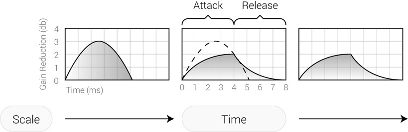
Figure 17.12 The input to the time stage arrives from the scale stage and denotes the provisional amount of gain reduction. The attack within the time stage slows down the gain reduction growth. Note that even when the input to the time function starts to fall (2.5 ms), the output still rises as the provisional amount of gain reduction is still higher than the applied amount. Only when the provisional amount falls below the applied amount (4 ms) does the latter start to drop. At this point, the attack phase ends and the release phase starts.
One crucial thing to understand is that attack and release are applied on gain reduction, and that the time stage, where these are applied, is unaware of the threshold setting. Many sources state incorrectly that the release only occurs when the signal level drops below the threshold. In reality, both the attack and release affect gain reduction (and in turn the signal level), even when the signal level changes above the threshold. Figure 17.13 demonstrates this.
Despite what many sources suggest, the release function is not related to the signal dropping below the threshold.
The top waveform in Figure 17.13 is known as a noise burst, and is commonly used to demonstrate the time function of dynamic range processors. However, it could be just as easily demonstrated using a voice rising from levels already above the threshold and then

Figure 17.13 Attack and release above the threshold. The top waveform rises from –6 to 0 dB, then falls back to –6 dB. This waveform passes through an Oxford Dynamics plugin with the shown settings, and the post-compression result is the bottom waveform. The compressor threshold is set to –12 dB (dashed lines) so all the level changes in the top waveform happen above the threshold. On the bottom waveform, which shows the output of the compressor, we can see the action of both the attack and release. Analog compressors behave in the same way.
![]()
Track 17.13: Noise Burst Low Threshold
A compressed version of Track 17.5, with the threshold set to –40 dB and ratio to maximum. You should hear the first attack when the noise rises to –12 dB, and then again when it rises to –6 dB (which happens above the threshold). When the noise falls back to –12 dB (a level above the threshold), the gain recovery caused by the release function is evident.
The following two tracks involve a threshold at –50 dB and a ratio of 1.5:1. Apart from the very first 300 ms and the closing silence, the vocal is always above the threshold. The only differences between the two tracks are the attack and release settings. There is no doubt that the two are distinctly different, demonstrating that both the attack and release affect level variations above the threshold.
Track 17.14: Vocal Compression I
Track 17.15: Vocal Compression II
Plugin: Sonnox Oxford Dynamics
falling back to levels above the threshold (something like ah-Ah-AH-Ah-ah, where only the ah is below the threshold). The fact that the attack and release affect level changes even when these happen above the threshold means that the dynamics are controlled to a far greater extent than they would be if compressors only acted when signals overshoot or drop below the threshold. The attack and release would still be applied on the AH just like on the Ah. Every so often, vocals do fluctuate in level after overshooting the threshold, and the release and attack still affect our ability to balance them. Also, attack and release will still act on signals fluctuating above the threshold, even when it is set very low.
Hold
Very few compressors provide a hold parameter, which is also linked to the time function. In simple terms, hold determines how long gain reduction is held before the release phase starts. Figure 17.14 illustrates this. In practical terms, the function of hold on a compressor is achieved by altering the release rate, so during its early stages gain reduction hardly changes. Although the results are only similar to those shown in Figure 17.14, the overall impression is still as if gain reduction is held.

Figure 17.14 The hold function on a compressor. This simplified illustration shows the input levels at the top, the amount of applied gain reduction in the middle, and the post-compression level at the bottom. We can see that once the original level drops, the compressor holds the gain reduction for a while before release.
Phase inverse
The phase stage in Figure 17.5 is shown for explanation’s sake—it might not be part of a real-world compressor. The output of the time stage is the final gain reduction, and it involves a positive magnitude (Figure 17.5e). What the gain stage expects is the amount of gain that should be applied on the signal, not the amount of gain reduction. So, in order to reduce the input level by 3 dB, the gain stage should be fed with –3 dB. In order to convert the gain reduction to gain, the magnitude of the former is mirrored around the 0 dB line using a simple phase inversion (Figure 17.5f).
Additional controls
Now that we have established the basic principles behind the operation of compressors, let’s take a look at a few more controls. Figure 17.15 shows the addition of the controls we will look at in the next sections.
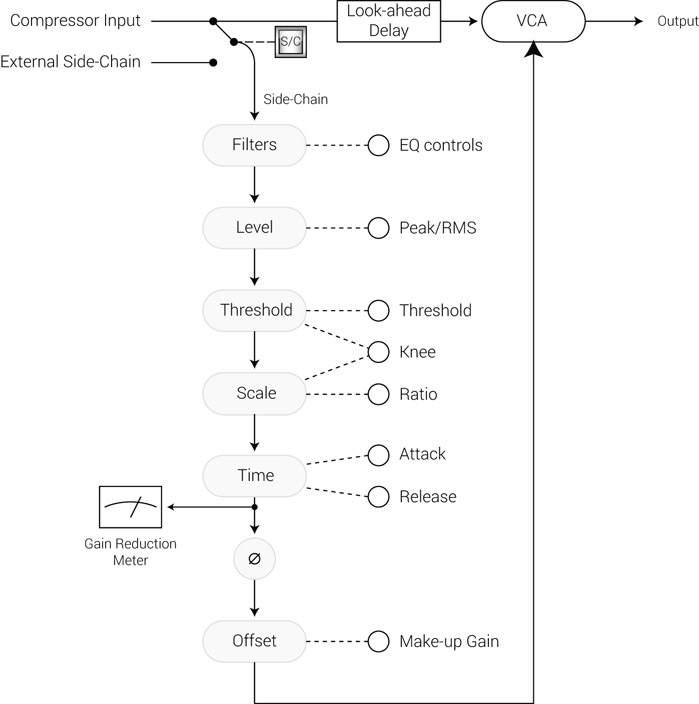
Figure 17.15 Detailed depiction of a compressor’s internal workings.
Makeup gain
A compressor’s principal function is to make louder sounds softer. As a result, the perceived loudness of the compressed signal is likely to drop. To compensate for this, the makeup gain control (sometimes called gain or output) simply boosts the level of the output signal by a set number of dBs. The boost is applied uniformly to the signal, independently of any other control setting—both signals below and above the threshold are affected. Compressors achieve this by either biasing the side-chain’s gain amount before it is applied by the gain stage or by simply amplifying the signal after the gain stage.

Figure 17.16 Makeup gain. (a) The input signal before compression. (b) The signal after compression with 2:1 ratio, but before makeup gain. (c) The output signal after 2 dB of makeup gain. Note that, in this example, the peak measurement of both the input (a) and the output (c) signals is identical. Yet (c) will be perceived as louder.
As per our louder-perceived-better axiom, when we do A/B comparisons, there is a likelihood that the compressed version will sound less impressive due to the loudness drop. Makeup gain is often set so that, whether the compressor is active or not, the perceived signal loudness remains the same. This way, any comparison made is fair and independent of loudness variations.
Some compressors have an automatic makeup gain. Compressors with auto makeup gain calculate the amount of gain required to level the input and output signals based on settings such as threshold, ratio, and release. The auto makeup gain is independent of the input signal and only varies when the compressor controls are adjusted. Arguably, there is no way an automatic makeup gain will match flawlessly the dynamics of all instruments and the possible levels at which these have been recorded. In practice, auto makeup gain often produces a perceived loudness variation when the compressor is bypassed. When able to do so, people will often choose to turn this function off.
Hard- and soft-knees
On the ratio curve, the knee is the threshold-determined point where the ratio changes from unity gain to the set ratio. It takes little imagination to see that it is so named because on a transfer characteristics graph, this curve is reminiscent of a sitting person’s knee. The type of compressors we have discussed so far work on the hard-knee principle— the threshold sets a strict limit between no treatment and full treatment. The sharp transition between the two provides a more evident compression and a more distinctive effect. We can soften such compression by lengthening the attack and release, but such settings do not always complement the compressed material.
The soft-knee principle (also termed over-easy or soft ratio) enables smoother transition between no treatment and treatment—gain reduction starts somewhere below the threshold with diminutive ratio, and the full compression ratio is reached somewhere above the threshold. While a hard-knee compressor toggles between 1:1 and 4:1 as the signal overshoots, on a soft-knee compressor the ratio gradually grows from 1:1 to 4:1 in a transition region that spreads to both sides of the threshold. This second exception for signals below the threshold being reduced in level is illustrated in Figure 17.17.
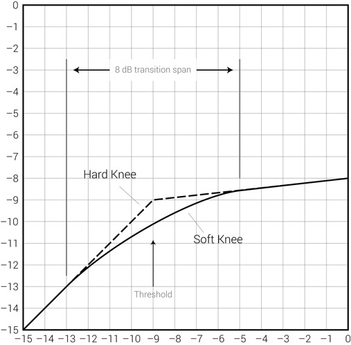
Figure 17.17 Hard- and soft-knees. With hard-knee, the ratio of compression is attained instantly as the signal overshoots. With soft-knee, the full ratio is achieved gradually within a transition region that spreads to both sides of the threshold.
Soft-knee is useful when we want more transparent compression (often with vocals). The smooth transition between no treatment and treatment minimizes the compression effect, which in turn lets us dial a higher ratio. Having soft-knee also frees the attack and release from the task of softening the compression effect and lets us dial shorter times on both (which can be useful for applications such as loudening). When we are after the compression effect, a hard-knee is more suitable.
Soft-knee for more transparent compression. Hard-knee for more effect.
Compressors might provide hard-knee only, soft-knee only, or a switch to toggle between the two. Some compressors also provide different degrees of knee rates, which let us determine the dB span of the transition region with relation to the input scale. For example, in Figure 17.17, the transition span is 8 dB, with 4 dB to each side of the threshold. The compression in this case will start with a gentle ratio at –13 dB, and the full ratio will be achieved at –5 dB. A transition span of 0 dB denotes hard-knee function (such a setting can be seen on the Oxford Dynamics plugin in Figure 17.13, below the attack control).
In order to produce soft-knee behavior, an analog compressor has to alter both the threshold and the scale functions. A precise soft-knee is difficult to achieve in the analog domain: the threshold might not fall within the center of the knee, and the ratio is likely to diverge outside the transition region. Digital compressors have no problem in exhibiting a perfect soft-knee like the one in Figure 17.17.
![]()
Track 17.16: Vocal Uncompressed
This uncompressed vocal track involves noticeable level variations.
Track 17.17: Vocal Hard-knee
Although the level fluctuations have been reduced, some still exist, mainly due to the operation of the compressor. The working compressor can be easily heard on this track.
Track 17.18: Vocal Soft-knee
Compression settings identical to the previous track, only with a soft-knee (40 dB transition span). The level fluctuations in the previous track are smoothened by the soft-knee, and the operation of the compressor is less evident.
One issue with soft-knee is that the compression starts earlier (below the threshold), and so does the attack. Since the attack starts earlier, less of the natural attack is retained. Therefore, soft-knee might not be appropriate when we try to retain the natural attack of sounds, and with it longer attack times might be needed. Notice the loss of dynamics, life, and some punch in the soft-knee version:
Track 17.19: Drums Hard-knee
Track 17.20: Drums Soft-knee
Plugin: Sonnox Oxford Dynamics
Drums: Toontrack EZdrummer
Look-ahead
Compression can be tricky with sharp level changes, like those of transients. In order to contain transients, a compressor needs a very fast response, but this is not always possible. For one, the gain stage of some compressors, optical ones for instance, is often not fast enough to catch these transients. Then, even if a compressor offers fast response times, the quick clamping down of signals might not produce musical results. It would be great if the side-chain could see the input signal slightly in advance so it could have more time to react to transients. The look-ahead function enables this.
One way to implement look-ahead on analog compressors is to delay the signal before it gets processed. The delay, often around 4 ms long, is introduced after a copy is sent to the side-chain (Figure 17.18). This way, a transient entering the compressor will be seen immediately by the side-chain, but will only be processed shortly after. This enables longer (more musical) attack times since there is a gap of a few milliseconds between the compression onset and the actual processing of the signal that triggered it. By way of analogy, if we could have look-ahead in tennis, it would be like freezing the ball for a while as it crosses over the net, so a player can perfectly reposition after seeing where the ball is heading.

Figure 17.18 A look-ahead function on a hardware compressor. After a copy is sent to the side-chain, the signal is delayed on the main signal path, giving the control circuit more time to respond to the signal.
On a hardware compressor, a look-ahead function will be switchable. When look-ahead is engaged, the output signal is delayed as well. These few milliseconds of delay rarely introduce musical timing outflow, but can lead to phase issues if the compressed signal is mixed with a similar track (snare top, snare bottom, for example). With software plugins, any delay that might be introduced is normally auto-compensated.
Stereo linking
A stereo hardware compressor is essentially a unit with two mono compressors. Unless otherwise configured, these two mono compressors work independently in what is known as dual-mono mode. Let us consider what happens when stereo overheads are fed into a compressor in such a mode. A floor tom is likely to be louder on the microphone that covers one side of the drum kit—say, the right side. When the tom hits, the right compressor will apply more gain reduction than its left counterpart. As a result, the left channel will be louder and the overheads image will shift to the left. Similarly, when the left crash hits, the overheads image will shift to the right. So, in dual-mono mode, every time a drum hits on either sides of the panorama, the stereo image might shift to the opposite side. Stereo linking interconnects both compressors so an identical amount of gain reduction is applied to both channels. With stereo linking engaged, as the floor tom hits, both sides are compressed to an identical extent and no image shifting occurs.
In all but a very few cases, stereo linking is engaged when a stereo signal is compressed.
There are various ways to achieve stereo linking. For example, the stereo input might be summed to mono before feeding both the left and right side-chains. The problem with this approach is that phase interaction between the two channels might produce a disrupted mono sum. To combat this, some compressors keep a stereo separation throughout the two side-chains and take the strongest-win approach—the heaviest gain reduction product of either channel is fed to the gain stage of both. With the strongest- win approach, it still makes sense to have different settings on the different channels— by setting a lower ratio on the right channel, we make the compressor less sensitive to right-side events (such as a floor tom hit).
![]()
Track 17.21: Drums Stereo Link On
The compression triggered by the tom causes the kick, snare, and hi-hats to drop in level, but their position on the stereo image remains the same.
Track 17.22: Drums Stereo Link Off
With stereo linking off, image shifting occurs. With every tom hit, the kick, snare, and hi-hats shift to the left. As the tom decays, these drums slowly return to their original stereo position.
Plugin: PSP Vintage Warmer 2
Drums: Toontrack EZdrummer
Unlike their hardware counterparts, software compressors rarely provide a stereo linking switch. A software compressor knows whether the input signal is mono or stereo, and, for stereo input, stereo linking is automatically engaged. Some compressors still provide a switch to enable dual-mono mode for stereo signals. Such a mode might be required when the stereo signal has no image characteristics, as in the case of a stereo delay.
External side-chain
By default, both the gain stage and the side-chain are fed with the same input signal. Essentially, the signal is compressed in relation to its own level. Most compressors let us feed an external signal into the side-chain, so the input signal is compressed in relation to a different source (Figure 17.19). For example, we can compress a piano in relation to the level of the snare. Hardware compressors have side-chain input sockets on their rear panel, while software sequencers let us choose an external source (often a bus) via a selection box on the plugin window. A switch is often provided to toggle between the external side-chain and the native, internal one. There is also usually a switch that lets us listen to the side-chain signal via the main compressor output (overriding momentarily the compressed output).

Figure 17.19 External side-chain. An external signal can feed the side-chain, so the compressor input is compressed with relation to an external source.
Side-chain filters and inserts
Quite a few compressors let us equalize the side-chain signal (the section to the right of the plot in Figure 17.4 is one example). As can be seen from Figure 17.5, such equalization occurs on the side-chain only (not the main signal path) and affects both the native and external side-chain sources. Some analog compressors also provide a side-chain insertion point, enabling processing by external devices. Soon we will look at the many applications for side-chain equalization.
Compressor meters
Three metering options are commonly provided by compressors: input, output, and gain reduction. When it comes to mixing, people often say, “Listen, don’t look.” True—we should be able to set all the compressor controls based on what we hear; but recognizing the subtleties in compressor action takes experience, and the various meters can often help, especially when it comes to initial rough settings. Fine and final adjustments are done by ear.
Out of the three meters, the most useful is the gain reduction meter, which shows the applied amount of gain reduction. The gain reduction reading combines the effect of all the compressor controls, for example threshold, ratio, attack, release, peak, RMS, etc. The main roles of this meter are:
- To teach us how much gain reduction is applied (which hints at the most suitable amount of makeup gain).
- To teach us when gain reduction takes place. Mostly we are interested in:
- – when it starts; and
- – when it stops.
- To provide a visual indication of the attack and release activity (which can help in adjusting them).
To give an example, when our aim is to balance the level of vocals, we want the gain reduction meter to move with respect to the level fluctuation that we hear on the unprocessed voice (or see on the input meter). If the attack or release is too long, the meter will appear lazy compared with the dynamics of the signal, and so might the compression.
The terms compression and gain reduction are often used interchangeably, where people think of the amount of compression as the amount of gain reduction. When people say they compress something by 8 dB, they mean that the gain reduction meter’s highest reading is 8 dB. Associating the gain reduction reading with the amount of compression is not a good practice, though. If the gain reduction meter reads steady at 8 dB (say, due to a hypothetical release time of 10 hours), no compression is taking place—there is simply constant gain attenuation of 8 dB. For the most part, such a compressor behaves like a fader—apart from when the gain reduction climbs to 8 dB, the output signal keeps all its input level variations, whether these happened above or below the threshold. In order for compression to occur, the amount of gain reduction must vary over time and the gain reduction meter must move; and the faster it moves, the more compression takes place. There is a similarity here to sound itself—sound is the outcome of changes in air pressure; steady pressure, whether high or low, does not generate sound. Likewise, the amount of compression is determined by changes in gain reduction. We might want to consider the amount of compression as an average of the absolute difference between the peak and RMS gain reduction. But that’s a story for a different book.
In addition, we should also consider the range within which this meter moves. If a vocal overshoots the threshold between phrases, but within each phrase the gain reduction meter only moves between 4 and 6 dB, then the effective compression is only 2 dB. At the beginning and end of each phrase, the signal is still compressed on its way to and back from 4 dB, but this compression is marginal compared with the compression taking place between 4 and 6 dB. We will call the range where gain reduction varies dynamic compression (4–6 dB in our case), and use the term static compression for the static range (0–4 dB in our case), where gain reduction only occurs on the way to or back from the dynamic compression. Figure 17.20 illustrates the differences between the two. Static compression can happen either as a result of slow release or a threshold being set too low. If the latter is the case, it might be wise to bring up the threshold, so the gain reduction meter constantly moves between 0 dB and the highest reading. This would minimize static compression. However, there are cases where static compression makes perfect sense, such as when compression is employed to shape the dynamic envelope of sounds and the threshold is set intentionally low to enable more apparent attack.
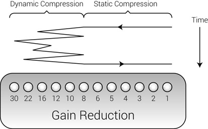
Figure 17.20 Dynamic and static compression. The dynamic compression happens in the range where the gain reduction meter varies. The static compression only happens as gain reduction rises to or falls from the dynamic compression range.
The subjective observation of light, moderate, or heavy compression is based on the gain reduction meter. We just saw that the amount of compression is far more complex than the basic reading this meter offers. It is also unsafe to translate any observations to numbers, as what one considers heavy the other considers moderate. We can generalize that 8 dB of compression on the stereo mix is quite heavy. For instruments, people usually think of light compression as somewhere below 4 dB, heavy compression as somewhere above 8 dB, and moderate compression as somewhere in between these two figures (Figure 17.21). We are talking about dynamic compression here—having 20 dB of constant gain reduction is like having no compression at all.
You might have noticed that the numbers in Figure 17.21 are positive and arranged from right to left. This is the opposite direction to the input and output meter, and suggests that gain reduction brings the signal level down, not up. Also, on compressors with no dedicated gain reduction meter, gain reduction is displayed on the same meter as the input and output levels (with a switch to determine which of the three is shown). Since on most meters the majority of the scale is below 0 dB, this is also where gain reduction is shown. Very often a gain reduction of 6 dB will be shown as –6 dB.

Figure 17.21 A gain reduction meter. The descriptions above the meter are an extremely rough guideline as to what some people might associate different amounts of gain reduction with.
![]()
To be technically correct, a decrease of a negative value is an increase, so a gain reduction of –6 dB essentially denotes a gain boost of 6 dB. Many designers overlook that, and, despite having a dedicated meter labeled “gain reduction,” the scale incorrectly shows negative values.
The input meter can be useful when we set the threshold. For example, if no signal exceeds –6 dB except for a peak we want to contain, this is where the threshold might go. We can also determine the action range of input levels by looking at this meter (more on action range below). The output meter gives a visual indication of what we hear and ensures that the output level does not exceed a specific limit, such as 0 dBFS. The output meter can also help us in determining rough makeup gain without having to toggle the compressor in and out.
Controls in practice
Threshold
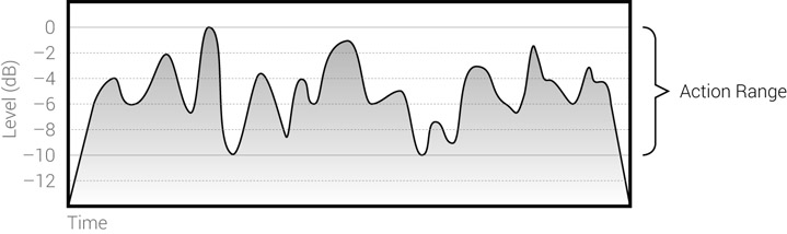
Figure 17.22 The action range of a non-percussive performance. Apart from the initial rise and final drop, the signal level is only changing within the 0 to –10 dB range.
Figure 17.22 shows possible levels of a non-percussive performance—a vocal phrase, perhaps. We can see that the levels fluctuate between the 0 and –10 dB range. We will call this range the action range and it can help us determine the threshold setting for specific applications. It should be made clear that setting the threshold anywhere above 0 dB has little point—unless the knee is soft, no compression will take place. Setting the threshold within this range will yield selective compression—only the signal portions above the threshold will be treated. Sometimes this is what we want, as when we only want to treat loud parts of the signal. However, the danger in selective compression is that the transition between treatment and no treatment happens many times, and the compression becomes more obvious. Setting the threshold to the bottom of the action range (–10 dB in Figure 17.22) will result in uniform treatment for all the level changes within it. While this might not be suitable with every compressor application, when a performance involves an evident action range, its bottom might provide a good starting point for threshold settings.
One key point to consider is what happens when we set the threshold below the action range. Say we first set the threshold to the bottom of the action range at –10 dB, and set the ratio to 2:1. The highest peak in Figure 17.22 hits 0 dB, so by overshooting 10 dB it will be reduced by 5 dB. Also, if we assume that the compressor timing rates are based on 10 dB and the release is set to 10 ms, as the same peak dives to –10 dB, it will take the 5 dB of gain reduction 5 ms to recover. Now if we reduce the threshold to –20 dB, the same peak overshoots by 20 dB and will be reduced by 10 dB—twice as much as before. Also, as the gain reduction is now 10 dB, it will take it 10 ms to recover. Effectively, by lowering the threshold we increase the amount of gain reduction, which results in further depression of dynamics. In addition, we slow down the release (and attack) response. Also, having the threshold at –20 dB will result in 5 dB of static compression as everything between –20 and –10 dB will be constantly compressed (apart from during the leading rise and closing fall).
Let us discuss three common compression applications and their threshold settings. These are containing peaks, level balancing, and loudening (condensing levels). Figure 17.23 shows the level of a hypothetical performance, say vocal. Each column represents a different application, and the threshold setting for each is shown on the top row. The top row also shows the input signal, which is identical in all three cases. In this specific performance, there is one peak and one level dip.
The left column (a) is concerned with containing levels. The high threshold is set around the peak base, above all other levels. The compression reduces the peak level, but no other portion of the signal. Reducing the peak lets us boost the overall level of the signal, and, by matching the original peak with the compressed one, moderate- and low-level signals are made louder. Note that in this case, the loss of dynamics is marginal.

Figure 17.23 Threshold settings for common compression applications. (a) Containing levels. (b) Balancing levels. (c) Loudening. The columns from top to bottom show the input signal and the threshold setting, then the compressed signal before makeup gain and the output signal after makeup gain.
![]()
The term containing levels is being used here as a more general term for containing peaks. Containing peaks is concerned with preventing levels from exceeding a predefined limit—a job for a limiter, really. We might want to contain the louder downbeats of a strumming guitar, although these might not peak.
The center column (b) demonstrates possible compression for level balancing. The threshold is set to a moderate level right above the dip, but below all other portions of the signal. The idea is to pull everything above the dip down toward it, which is exactly what happened after compression. Note, however, that compared with the compression shown on the left column, the signal has lost more of its dynamics. The makeup gain offsets the signal, so moderate levels are back to their original area (around the middle line of the input graph). If we look at the output graph, we can see that the peak got pulled down toward this middle line, while the dip got a gentle push up from the makeup gain. Again, one possible issue with this technique is the uneven compression effect it deposits due to selective compression—the dip gets louder, but as opposed to the rest of the signal its dynamics remain unaffected. If the applied compression results in audible effect, it will not be evident on the dip. To overcome this, we can lower the threshold so even the dip gets a taste of the compressor effect.
The right column (c) exhibits a compression technique used when we wish to make instruments louder or when we want to condense their dynamics. The low threshold is set at the base of the signal, so all but the very quiet levels get compressed. Two things are evident from the post-compression graph. First, the levels are balanced to a larger extent as the dip was treated as well. After compression, the peak, dip, and moderate levels are highly condensed. Thus, this technique can also be used for more aggressive level balancing. Second, we can see that the signal has dropped in level substantially. To compensate for this, makeup gain is applied to match the input and output peaks. In this case, the output signal will be perceived as louder than the input signal, since its average level rose by a fair amount. The main issue with this technique is that, of all three applications, it led to the greatest loss of dynamics.
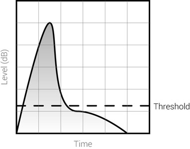
Figure 17.24 Catching the attack of a snare. The threshold is set so the attack is above it but the decay is below.
There is more to threshold settings than these general applications. Sometimes we know which part of an instrument’s dynamic envelope we should treat. On a snare, for example, it might be the attack, so the threshold is set to capture the attack only. Figure 17.24 illustrates this. One important thing to note is that the lower the threshold, the sooner we catch the attack buildup. In turn, this lets us lengthen the attack time, which, as we shall soon see, is often beneficial.
Ratio
A compressor with ratios above 10:1 behaves much like a limiter—with a 10:1 ratio, a signal overshooting by a significant 40 dB is reduced to a mere 4 dB above the threshold. Yet, even a compressor with ∞:1 ratio is not really a limiter (signals can still overshoot due to long attack or the RMS function), so ratios higher than 10:1 have a place in mixes. Mastering ratios (on a compressor before the limiter) are often gentle and kept around 2:1. Mixing ratios can be anything—1.1:1 or 60:1. Yet the ratio 4:1 is often quoted as a good starting point in most scenarios.
Logic has it that the higher the ratio, the more the compression applied and the more obvious its effect. One important thing to understand is that the degree of compression diminishes as we increase the ratio. As can be seen in Figure 17.25, turning the ratio from 1:1 to 2:1 for an 8 dB overshoot results in gain reduction of 4 dB. Turning the ratio from 8:1 to 16:1 for the same overshoot only results in an additional gain reduction of 0.5 dB. A more practical way to look at this is that changes of lower ratios are much more significant than the same changes for higher ratios—a ratio change from 1.4:1 to 1.6:1 will yield more compression than a ratio change from 8:1 to 16:1. Most ratio controls take this into account by having an exponential scale (for example, 1:1 to 2:1 might be 50% of the scale; 2:1 to 4:1 will be an additional 25%, and so forth).

Figure 17.25 The diminishing effect of increasing the ratio. The ratio is shown above each graph. The threshold is set to 0 dB.
![]()
A demonstration of the diminishing effect of increasing the ratio can be heard in Track 17.3 (Rising Ratio). The majority of level lost and the increasing effect of compression is mostly evident in the first bar, where the ratio rises from 1:1 to 2:1, and in the second bar, where the ratio further rises to 4:1. The change in the following bars is marginal compared to the change in these first two bars.
We can make some assumptions as to the possible ratios in the three applications discussed in Figure 17.23. In the first case—containing levels—a high ratio, say 10:1, might be suitable. With the high threshold set to capture the peak only, the ratio simply determines the extent by which the peak is brought down, with a higher ratio being more forceful. In the second case—balancing levels—the moderate threshold is set around the average level. The function of the ratio here is to determine the balancing extent. Since most of the signal is above the threshold, a high ratio would result in a noticeable effect and possible oppression of dynamics. However, a low ratio might not give sufficient balancing, so a moderate threshold, say 3:1, could be suitable here. In the third case— loudening—the low threshold already sets the scene for some aggressive compression. Even a moderate ratio can make the compression so aggressive that it will suppress dynamics. Therefore, a low ratio, say 1.4:1, might be appropriate.
The relationship between threshold and ratio
In the three examples above, the lower the threshold, the lower the ratio, which brings us to an important link between the two controls. Lowering the threshold means more compression, while lowering the ratio has the opposite effect. Often these two controls are fine-tuned simultaneously, where lowering one is followed by the lowering of the other. Ditto for rising. The idea is that once the rough amount of required compression is achieved, lowering the threshold (more compression) and then lowering the ratio (less compression) will result in roughly the same amount of compression, but with a slightly different character.
Although lower threshold and higher ratio each result in more compression, the effect of each is different. Lower threshold results in more compression as larger portions of the signal are compressed. High ratio results in more compression on what has already been compressed. Put another way, lower threshold means more is affected, while higher ratio means more effect on the affected. If the threshold is set too high on a vocal take, even a ratio of 1,000:1 will not balance out the performance. If the ratio is set too low, the performance will not balance, no matter how low the threshold is. Finding the right balance between threshold and ratio is one of the key nuts to crack when compressing.
Threshold defines the extent of compression. Ratio defines the degree. The two are often fine-tuned simultaneously.
This might be the right point to talk about how the two are utilized with relation to how evident the compression is. We already established that the threshold is a form of discrimination between what is being treated and what is not. In this respect, the higher the threshold, the more the discrimination. We can consider, for example, the compression of vocals, when our task is to make it as transparent as possible. Chances are that, with moderate threshold and moderate ratio, the effect of compression would be more evident than if we set the threshold very low but applied a very gentle ratio: 1.2:1, for example (Figure 17.26). Since we already established that the attack and release are also applied on level changes above the threshold, we know that the timing characteristics are applied even if the threshold is set very low. All of this is said just to stress that lower threshold does not necessarily mean more evident effect—this is determined by both the threshold and the ratio settings, as well as other settings described below.

Figure 17.26 The effect of compression with relation to the threshold and ratio settings. The scale in these graphs represents the full dynamic range of the input signal. (a) Moderate threshold and ratio. One should expect more evident compression here as the threshold sets a discrimination point between untreated signals and moderately treated signals. (b) Low threshold and ratio. One should expect less evident compression here as all but the very quiet signal will be treated gently.
Attack
One reason for longer attack times was given earlier—to prevent the suppression of an instrument’s natural attack. But we don’t always want to keep the natural attack. Sometimes we want to soften a drum hit so kicks, snares, and the like are less dominant in the mix. In such cases, shorter attack is dialed.
The longer the attack time, the more we retain the instrument’s natural attack. However, this is not always wanted.
The way longer attack helps to retain the natural attack is easily demonstrated on percussive instruments. Figure 17.27 illustrates the effect of different attack times on a snare. We can see that, with no attack, the natural attack is nearly lost as the compressor squashes it down quite drastically (clearly, this is also dependent on the threshold and ratio settings). Then, the longer the attack, the more of the natural attack is retained. Long attack hardly affects the natural attack—or, in this specific snare case, hardly affects anything at all.
We might instinctively think: If we want to retain the natural attack of an instrument, why not just set the attack time as high as possible? The long attack in Figure 17.27 demonstrates why this is unwise. We can see that, by the time the signal has dropped below the threshold, the attack has barely built up to cause any significant gain reduction— it nearly canceled out the compression effect, making the whole process rather pointless. Based on Figure 17.12, we know that, shortly after the snare signal starts to drop, the applied gain reduction also starts to drop, and at this point the attack phase stops and the compressor enters the release phase. This point on Figure 17.27 is where the attack buildup turns gray, and we can see that the potential full effect is not achieved for either the medium or the long attack settings.
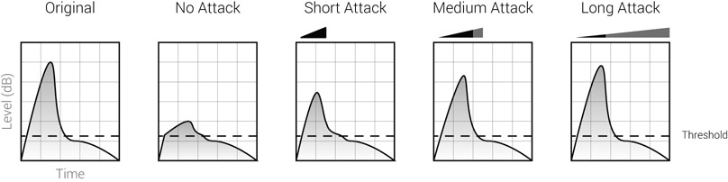
Figure 17.27 Different attack times on a snare. The attack buildup is shown below each caption. The longer the compressor attack time, the more of the instrument’s natural attack is retained.
![]()
Track 17.23: Snare Uncompressed
The original snare track used for the following samples. For the purpose of demonstration, the compressor threshold in the following tracks was set to –15 dB and the ratio to ∞:1.
Track 17.24: Snare Attack 10 ms
The extremely short attack on the compressor immediately reduces the natural attack of the snare, simply resulting in overall level reduction.
Track 17.25: Snare Attack 1 ms
With 1 ms of attack, the result is not much different from in the previous track. Yet, a very small part of the natural attack manages to remain, so there is a notch more attack on this track.
Track 17.26: Snare Attack 10 ms
10 ms is enough for a noticeable part of the natural attack to pass through, resulting in compression that attenuates the late attack and the early decay envelopes.
Track 17.27: Snare Attack 50 ms
An even larger portion of the natural attack passes through here, resulting in gain reduction that mainly affects the decay.
Track 17.28: Snare Attack 100 ms
100 ms of attack lets the full natural attack through. Essentially, little gain reduction is applied and it affects the early decay envelope. Compared to the uncompressed track, a bit of the early decay was reduced in level here.
Track 17.29: Snare Attack 1000 ms
The majority of sound in each of these snare hits is no longer than 500 ms. 1 second is too long for the compressor to respond, so no gain reduction has been applied at all, resulting in a track that is similar to the uncompressed one.
Plugin: PSP MasterComp
Drums: Toontrack EZdrummer
Even when the signal remains above the threshold after the attack phase, a longer attack time is rarely beneficial. We can demonstrate this on the piano key hit in Figure 17.28. The short attack brings the gain reduction to full impact slightly after the natural attack has declined, and the resultant dynamic envelope resembles the input signal envelope. This is not the case with the long attack, which clearly altered the dynamic envelope and resulted in unwanted timbre alteration. This example teaches us what is very likely to be a musical attack time for instruments of a percussive nature: one that only affects the natural attack without altering the dynamic envelope succeeding it.
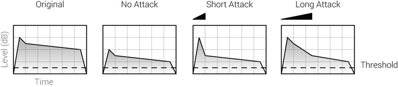
Figure 17.28 Different attack times on a piano key hit. The long attack time caused alteration of the level envelope, which would distort the timbre of the instrument.
Another reason why a longer attack would be beneficial involves the compression of overheads. If the kick is the main instrument to trigger the compression and the attack is set too short, not only the kick’s natural attack but also any other drum played underneath it (such as the hi-hats) would be suppressed. If this happens on the downbeat, downbeat hats would be softer than other hats. This might be suitable with more exotic rhythms, but rarely for the contemporary acid-house track, punk-rock, gangsta rap, or just about anything else. A longer attack will let the downbeat hats sneak in before the compressor acts upon them.
One of the things we have to consider when it comes to attack times is how much gain reduction actually takes place. The more gain reduction there is, the more noticeable the attack will be—there is no comparison between an attack on maximum gain reduction of 1 dB and that of 8 dB. Generally speaking, heavy gain reduction could benefit from longer attack times, so large upswings take place gradually rather than promptly, making level changes less drastic. In addition, fast attack and serious gain reduction can easily produce an audible click. Although such attack clicks are sometimes used to add definition to kicks, they are mostly unwanted.
Nevertheless, there is a catch-22 here since a longer attack lets some of the level through before bringing it down (and with heavy compression it is quite a long way down). So with longer attack times level changes might be less drastic but more noticeable. This is often a problem when heavy compression is applied on less percussive sounds such as vocals.
![]()
Track 17.30: Drums Uncompressed
The uncompressed version of the drums used in the following samples.
Track 17.31: Drums Attack 5 ms
Notice how the hi-hats’ level is affected by the compression applied on the kick and snare. Also, the short attack suppresses the natural attack of both the kick and the snare.
Track 17.32: Drums Attack 16 ms
16 ms of attack is enough to prevent the kick and snare compression from attenuating the hats. In addition, the natural attack of both these drums is better retained.
Plugin: McDSP Compressor Bank CB1
Drums: Toontrack EZdrummer
Track 17.33: Vocal Attack 1 ms
This very short attack time yields instant gain reduction, which makes the compression highly noticeable. Essentially, each time the voice shoots up, a quick level drop can be discerned.
Track 17.34: Vocal Attack 5 ms
5 ms of attack means that the gain reduction is applied more gradually, producing far fewer level fluctuations due to the operation of the compressor. This attack time is also short enough to reasonably tame the vocal upswings.
Track 17.35: Vocal Attack 7 ms
There are still some quick gain reduction traces in the previous track, and 7 ms of attack reduces these further. However, the longer attack means that the voice in this track manages to overshoot higher.
Track 17.36: Vocal Attack 30 ms
30 ms is too long, and the compressor misses the leading edge of the vocal upswings. In addition, the compressor does not track the level variations of the vocal, making level fluctuation caused by the compressor more noticeable.
Track 17.37: Vocal Attack Pop
This track is also produced using 30 ms of attack, but with lower threshold and higher ratio so as to draw heavier gain reduction. Profound level pops can be heard on “who,” “running,” and “pass.”
Plugin: Sonnox Oxford Dynamics
If the attack is too short, the vocal dynamics flatten, but if the attack is made longer, there might be a level pop on the leading edge of each phrase. It is sometimes possible to find a compromise in these situations, and, when suitable, raising the threshold or lowering the ratio can also help. Yet, a few compressor tricks described later in this chapter can give a much more elegant solution and better results.
Another consequence of fast attack is low-frequency distortion, the reason being that the period of low frequencies is long enough for the compressor to act within each cycle rather than on the overall dynamic envelope of the signal. Figure 17.29 shows the outcome of this, and we can see the attack affecting every half a cycle. The compressor has reshaped the input sine wave into something quite different, and as a result distortion is added. The character of such distortion varies from one compressor to another, and it can be argued that analog compressors tend to generate more appealing distortion. In large amounts, this type of distortion adds rasp to the mix. But in smaller, more sensible amounts, it can add warmth and definition to low-frequency instruments, notably bass instruments.
The main purpose of the hold control is to rectify this type of distortion. By holding back the gain reduction for a short period, the attack and release are prevented from tracking the waveform. The cycle of a 50 Hz sine wave is 20 ms; often the hold time is set around this value.
The attack settings can affect the tonality of the compressed signal, where longer attack times tend to soften high frequencies. Alternatively, this can be seen as low-frequency emphasis and added warmth. The reason for this is demonstrated in Figure 17.30. High frequencies are the result of quick level changes, and low frequencies are the result of slow ones. A long release can slow the rate at which the signal level rises, which softens the quick level rise of high frequencies.

Figure 17.29 Low-frequency distortion resulting from fast attack settings. The top track is a 50 Hz sine wave passing through the McDSP Analog Channel 1 shown on the bottom right. The compressor setting involves 1 ms of attack and 10 ms of release. The rendered result is shown on the bottom track, where we can see the attack acting within each half cycle.
![]()
Track 17.38: Bass Uncompressed
The source bass track used in the following tracks.
Track 17.39: Bass LF Distortion Fast TC
The low-frequency distortion was caused by the fast attack (10 µs) and fast release (5 ms).
Track 17.40: Bass LF Distortion Fast Attack
Although the release is lengthened to 100 ms, the 10 µs attack still produces some distortion. When a bass is mixed with other instruments, a degree of distortion as such can add definition and edge.
Track 17.41: Bass LF Distortion Slow TC
With the release at 100 ms and the attack lengthened to 2 ms, there is only a faint hint of distortion.
Plugin: Digidesign DigiRack Compressor/Limiter Dyn 3
Release
Release and attack have a few things in common. A very short release can also distort low frequencies for the same reason a short attack can. Here again, the hold control can reduce this type of distortion. Long release tends to soften high frequencies on the same principle that long attack does. A very short release can cause audible clicks, although, in contrast to attack clicks, it is hard to think of any practical use for these release clicks. Release settings also become somewhat more important with heavier compression, as the release is applied on larger amounts of gain reduction.
Short release times can cause low-frequency distortion and audible clicks.

Figure 17.30 Level change rate and frequencies. (a) We can see that the slope of the high-frequency waveform is steeper. By the time the high-frequency sine wave had risen by 20 dB, the low-frequency sine wave had only risen by 10 dB. (b) Faster level changes are associated with high frequencies. A long attack on a compressor can turn a level rise like (2) into (3), which softens high frequencies. We will see later that a gate can result in an abrupt level jump like (1), which generates high frequencies.
![]()
Track 17.42: Bass LF Distortion Fast Release
The distortion on this track is the result of a fast release of 5 ms and a relatively long attack of 2 ms.
Plugin: Digidesign DigiRack Compressor/Limiter Dyn 3
One thing we have to consider is that the gain recovery during the release phase sometimes happens during silent sections. For example, if you try to sing aloud “when we eat” and then “when we go,” it is likely that you will cut the “eat” while fading out the “go.” Quick vocal drops such as “eat” can be shorter than 50 ms, and a release longer than that period might end up affecting silence. Although the release setting is important to control vocal drops, we have to acknowledge that some of the gain recovery can happen on inaudible sections. This suggests that the release can be more important for instruments that rarely dip into silence, such as overheads and rhythm guitars. These types of instruments are also more likely to experience pumping, which is caused by short release times.
Short release can cause pumping.
As per the discussion of the difference between gain reduction and compression, we know that a very long release time (hypothetically, 10 hours) will cause steady gain reduction, which is exactly the opposite of compression. Both long attack and long release slow down changes in gain reduction, which makes a compressor more of a fader. Subsequently, the effect of compression becomes less noticeable. By way of analogy, if during manual gain-riding the engineer’s fader movements are extremely slow, the input level variations will hardly alter. The true effect of compression only happens when the gain reduction tracks change in input levels. Short release times result in faster gain recovery, which in turn increases the average output level and the perceived loudness.
Short release times result in more compression, more evident effect and loudness increase.
![]()
Two compressed versions of Track 17.30. Note that the compression is more evident in the short-release version, which might also be perceived as louder. With 2,000 ms of release, most of the gain reduction is static, and the result is very similar to the uncompressed version.
Track 17.43: Drums Release 50 ms
Track 17.44: Drums Release 2000 ms
Plugin: Focusrite Liquid Mix (Trany 1a emulation) Drums: Toontrack EZdrummer
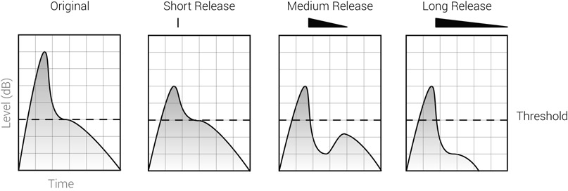
Figure 17.31 Release times on a snare. With short release, the decay is unaltered compared to the original signal. With medium release, it takes some time for the gain to recover, and only then the natural decay returns to its original levels. With long release, the decay is attenuated and very little of it is retained.
The previous attack section started with a snare demonstration, so let us start by using a snare to demonstrate the function of release. We established that the longer the attack is, the more the natural attack is retained. The effect of release can easily be misunderstood as it is exactly opposite in nature—the longer the release, the less natural decay is retained. The release control determines the rate at which the gain reduction can drop, or, in other words, how quickly the gain recovers. Once the input signal level drops, a longer release will slow down the recovery rate, so more gain reduction will be applied on signals. This effect was demonstrated in Figure 17.11 on a noise burst; Figure 17.31 shows this happening on a snare. It is interesting to note the effect of medium release, which quite noticeably reshapes the decay. This extra bump could alter the timbre of a snare in an unflattering way. So often we seek to either leave the decay as is or attenuate it altogether.
![]()
The following tracks demonstrate the effect of different release times. In all of them, 50 ms of attack allows most of the natural attack to pass through, leaving the gain reduction to mainly affect the decay of the snare. The longer the release, the slower the gain recovers, and consequently the more the decay is attenuated.
- Track 17.45: Snare Release 100 ms
- Track 17.46: Snare Release 500 ms
- Track 17.47: Snare Release 1000 ms
- Track 17.48: Snare Release 2000 ms
- Track 17.49: Snare Release 3000 ms
Note that in Track 17.46, it is possible to hear the decay recovering after being reduced in level straight after the attack. This is a demonstration of decay reshaping similar to that caused by the medium release shown in Figure 17.31.
Plugin: PSP MasterComp
Drums: Toontrack EZdrummer
In the case of vocals, we might want fast release so that the already dropping signal is not attenuated further by the compressor. But both attack and release are also concerned with level changes above the threshold, so in the case of vocals their function is often more concerned with tracking level fluctuations. As already suggested, the two are set to be fast enough to track these fluctuations.
Longer release on a compressor means less of the instrument’s natural decay and can cause timbre alterations.
No discussion about the release control would be complete without mentioning its strong link to the rhythmical nature of the song. When compression is applied on instruments with a percussive nature, the release dictates the length of each hit and how it decays. Different release settings can make a world of difference to how an instrument locks to the natural rhythm of the music. For example, a snare that hits every half-note might feel right in the mix if its perceived length is set to a quarter-note. There are no hard and fast rules—we have to experiment with the release settings until it feels right.
After a snare hit, the gain reduction meter shows when (and if) gain reduction falls back to 0 dB. Usually, we want this to happen before the next snare comes along, or the next hit will be attenuated by the ongoing gain reduction (Figure 17.32). One would naturally ask: But what happens if the drummer plays half-notes for the most part, and just before each chorus plays eighth-notes? A release setting that fits the length of a half-note will be too long for eighth-notes and will de-emphasize them. Chances are that these eighth-notes are there to squeeze some excitement in before the chorus, so such a de-emphasis is contrary to what we want. However, setting the release to fit eighth-notes might not be suitable for the half-notes, which are played for most of the song. As always, there are two main options here: either compromise on a setting that will be neither perfect nor horrible on both note lengths, or simply automate the release so all the hits feel right.

Figure 17.32 Release and snare spacing. (a) With slow release, the gain reduction does not recover before the next snare hit, causing attenuation to the consecutive hits and softening their attack. (b) With fast release, the gain reduction is back to 0 dB before the next hit, so the compressor treats all hits uniformly.
![]()
These two tracks demonstrate the effect release can have on the groove of rhythmical material. The effect might be easier to comprehend if one tries to conduct or move the head in relation to the beat.
Track 17.50: Drums Release Groove I
The long release on this track results in gain reduction that does not track the groove of the drums. The relatively slow gain recovery interferes with the natural rhythm.
Track 17.51: Drums Release Groove II
A shorter release setting yields compression that is much more faithful to the rhythm.
Plugin: Digidesign Smack!
Drums: Toontrack EZdrummer
In the case of percussive performance, we want gain reduction to fully drop before the next note arrives.
![]()
Track 17.52: Snare II Uncompressed
In this uncompressed version, the velocity of each snare hit is identical.
Track 17.53: Snare II Release 1000 ms
With 1 second of release, the gain never fully recovers between the various snare hits. Notice how the first hit is louder than all other hits, and how the last hit, which is the closest to the hit preceding it, is the quietest of them all.
Plugin: Sonnox Oxford Dynamics
Drums: Toontrack EZdrummer
Peak vs. RMS
Compared to peak sensing, an RMS compressor responds more slowly to changes in the input signal levels. In a way, the RMS averaging is a form of attack and release that is applied before the threshold stage. Having a strong link to the way we perceive loudness, RMS is very useful for instruments with a less percussive nature, such as vocals. However, their slow response makes them somewhat less suitable for percussive instruments, which change in level very quickly. If catch me if you can is the name of the game, a compressor will do a better job in peak mode.
Peak can work better on a percussive performance.
Since the RMS function slows quick level changes, the whole compression happens in a more relaxed manner that makes the compressor less evident. Peak level detection leads to more obtrusive operation and often more aggressive results. If aggression or power is what we are after, peak mode can be the right choice. If transparency or smoothness is our aim, RMS comes in handy. That being said, some RMS compressors can be very aggressive, powerful, and punchy, while a compressor in peak mode can also do a decent job on vocals.
RMS for transparency, peak for a firmer control and more effect.
![]()
Peak-sensing allows the compressor to respond much quicker to transients. This might lead to extra loss in dynamics, for example when compressing drums. Notice the loss of dynamics, attack, and punch in the peak version.
Track 17.54: Drums RMS
Track 17.55: Drums Peak
In the tracks above, no settings have changed apart from the Peak/RMS parameter. This makes the comparison somewhat unfair since the peak version would natively present a harder, more evident compression. The next track involves the same settings as in Track 17.55, only with a longer attack; the result is very similar to the RMS version.
Track 17.56: Drums Peak Longer Attack
Plugin: Cubase Compressor
Drums: Toontrack EZdrummer
Side-chain control
The interaction between the threshold, ratio, attack, and release gives us extensive control over the compressed signal. The ability to alter the side-chain signal adds further control and a few more compression applications. The side-chain signal can be altered via two facilities: either the built-in side-chain filters or any processors we apply on the external side-chain. Applying processors of our choice on the external side-chain gives us ultimate control. Yet, in some cases, the built-in filters suffice.
The nature of the signal feeding the side-chain can be one of two: the original input, which we can equalize, or a different signal altogether. The latter is used for specific applications or as part of a unique effect. More on this soon. For now, let us see the benefits of modifying the original input.
One of the main characteristics of compressors is that they are more responsive to low frequencies. Put another way, low frequencies tend to excite compressors more than high frequencies. One reason for this is that due to their long period, low-frequency signals spend more time above the threshold. Another reason is the fact that low frequencies have to be louder in order to be perceived as loud as higher frequencies (as per the equal loudness curves). This characteristic of low frequencies is the very reason why compressors have a reputation for dulling sounds—as low frequencies are being compressed, the level of high frequencies is also reduced.
Low frequencies tend to trigger compression more than high frequencies, a fact that can yield dulling of compressed instruments.
To give a practical example, when overheads are compressed, the kick is most often the first drum to trigger the compression. So, whenever the kick hits, the cymbals are also reduced in level. In addition, if the threshold is set too low (or the ratio too high), we could defeat the kick. However, settings that are appropriate for the kick might not trigger any compression when the cymbals are played. Effectively, not all of the drum kit is being compressed uniformly. A typical consequence of this is crashes that drop in level in a steplike fashion every time the kick or the snare hits (this is often something we check when compressing overhead, and both the attack and release can affect this behavior). The same issue exists with any type of broadband sound—low and high frequencies are not compressed to the same extent. The way to solve this is to apply some low-frequency filtering on the side-chain. By applying, for example, an HPF, we make the compressor response more balanced to broadband signals such as overheads.
A high-pass filter on the side-chain can bring about more uniform compression of broadband material.
![]()
Track 17.57: Drums II Uncompressed
The source track for the following samples.
Track 17.58: Drums II No SC Filter
The compressor is set to the fastest attack and release in order to draw the most obvious effect. Both the kick and snare trigger heavy and fast changes in gain reduction, which yields fluctuation in the crashes’ level.
Track 17.59: Drums II SC Filter
A 24 dB/oct HPF at 2 kHz is set to filter the side-chain. This essentially means that the kick does not trigger gain reduction anymore. Notice how the crashes’ level is smoother as a result. As one would expect, filtering the low frequencies from the side-chain yields less gain reduction, so in this track the threshold was brought down and the ratio up, so the gain reduction meter closely hits the same 10 dB as in the previous track.
Track 17.60: Drums II SC Only
This is the filtered SC signal that triggered the compression in the previous track.
Plugin: McDSP Channel G
Drums: Toontrack EZdrummer
Then there is also an issue with a performance that varies in pitch. We can give the example of vocals. The low-mids of a vocal performance vary noticeably with relation to the pitch being sung. As the melody travels up and down, the lower notes trigger more compression.
The higher-mids of a vocal performance tend to provide more solid energy, which is less dependent on the sung pitch. Applying an HPF on the vocals’ side-chain can yield more consistent compression. Perhaps the best demonstration of this problem has to do with bass guitars. The low E on a bass guitar (41 Hz) produces radically more low energy than the E two octaves above (165 Hz); therefore, the low E triggers more compression. Notwithstanding, the higher E will be more defined as its fundamental and harmonics start higher on the frequency spectrum. Having the low E less defined yet more compressed suggests how imbalanced the bass might sound. We can give the same example with the violin, trumpet, or virtually any instrument—the lower the note, the more the compression. Equalizing the side-chain can improve the compressor response to different notes. The actual filter being applied is often a high-pass filter (which can be of any slope), but low shelving equalizers can also be suitable for this purpose. Sometimes even a parametric EQ will work.
Side-chain equalization, more specifically low-frequency filtering, can yield more uniform compression for different notes.
There is another way to look at the above—if all frequencies below 500 Hz are filtered from the side-chain, the same frequencies are likely to be louder as they trigger less compression. If we boost 4 kHz on the side-chain, 4 kHz will be attenuated more (this is de-essing, in essence). This leads to an interesting phenomenon—equalizing the side-chain affects the tonality of the compressed signal. Generally speaking, one should expect the opposite effect to the settings dialed on the side-chain EQ. But the applied tonal changes are far more sophisticated than simply being the opposite of the side-chain EQ—it is compression-dependent equalization, otherwise a form of dynamic equalization. Apart from having to consider how the side-chain equalization affects the tonality of the compressed signal, we can use it to fine-tune the frequency spectrum of instruments. It takes experience to master this technique, but it could be worth the effort.
Side-chain equalization alters the tonality of the compressed signal and enables dynamic equalization that is more sophisticated than the standard static equalization.
Applications
The following is a summary of compressor applications:
- making sounds bigger, denser, fatter;
- accentuating the inner details of sounds;
- adding warmth;
- containing levels;
- balancing levels;
- loudening;
- softening or emphasizing dynamics;
- reshaping dynamic envelopes;
- adding punch;
- accenting the natural attack;
- accenting transients;
- reviving transients;
- reconstructing lost dynamics;
- emphasizing or de-emphasizing decays;
- moving instruments forward or backward in the mix;
- making programmed music sound more natural;
- applying dynamic movement;
- ducking;
- de-essing; and
- applying dynamic equalization.
Along with the new applications listed here, some of the applications already discussed are covered in greater depth in the coming sections.
Accentuating the inner details of sounds
Compression invariably condenses the levels of signals. One reason we find the effect so appealing is that it tends to emphasize the inner details of sounds. The small nuances of any performance—the lip movements of the vocalist or the airflow from a trumpet—become clearer, which is largely satisfying. Like anything in mixing, overdoing can have a countereffect. It is like luminance: in the right amount, it can enhance an image and make its details clearer, but too much of it results in blinding white.
Balancing levels
Figure 17.33 shows the possible levels of three mix elements before and after compression. We can see that before compression, the level fluctuations of the different instruments are quite problematic: at points the snare is the loudest, at points the bass, at points the vocals; the snare level varies; and sometimes the bass is louder than the vocals, sometimes vice versa. It’s a complete mess. No matter how much we try to balance such an arrangement using faders, the relative levels will always change over time and will do so quite radically. However, after we compress each instrument, we can balance them so their relative levels are consistent. Moreover, we can make them closer in level to one another, giving the impression of a louder, more solid mix.
Balancing of this sort usually happens very early in the mixing process, so as to make the tracks more manageable and instill some sense into their relative levels. Usually, we are not very fussy at this stage about perfecting the compression—rough settings would suffice to give reasonable balancing. As we progress from coarse to fine, we give more attention to the individual compression applied on each instrument.
Out of the three instruments shown in Figure 17.33, balancing the vocals is of prime importance as they exhibit the wildest level variations. Perhaps when working on the snare, balancing the level might be the second objective after adding punch. The level balancing approach of each instrument is likely to be different—we might want the vocal compression to be transparent while drawing more effect from the snare compression. If we have to generalize about sensible settings for level balancing, the following guidelines provide a possible starting point:
- Threshold—set at the bottom of the action range, so all level fluctuations are captured.
- Ratio—dependent on the extent of overshoots and to what degree we want to retain dynamics. High ratio can squash an instrument, while low ratio might not be sufficient to balance the levels. In Figure 17.33, chances are that the highest ratio will be applied on the vocals as they vary in level quite noticeably. Also, vocals have more settled dynamics, so softening these will be less noticeable.

Figure 17.33 Relative levels before and after compression. (a) Before compression the fluctuations in level make these three instruments impossible to balance. (b) After compression the balancing task is easier.
- Attack and release—set to fast for less-percussive instruments, so more compression is applied and level changes are quickly tracked. At the same time, we must observe low-frequency distortion and how the natural attack and decay are affected. For percussive instruments, we have to set longer attack and release to keep the dynamics.
- Hold—if available, can help reduce low-frequency distortion while letting us shorten the attack and release times.
- Knee—soft, as mostly when balancing levels we are not after the effect of compression.
- Level detection—depends on the instrument. Probably RMS for the vocals and peak for the snare.
- Side-chain filter—likely. Attenuating or filtering the side-chain lows of all three instruments can bring about more accurate results.
- Makeup gain—set so A/B comparison is fair (i.e., the perceived level will not change as we bypass the compressor).
One decision we often have to make is to what extent balancing should be done. If all the snare and kick hits are at the same level, they could sound like the product of a drum machine. Fortunately, the timbre of a drum changes in relation to the hit velocity, so some natural stamp is retained even if the individual hits are even in level. Yet, a more natural production could benefit from a relaxed balancing approach. In more powerful productions or more powerful sections of productions, many mixing engineers tend to even out the drum hits in a near mechanical fashion. We have to remember that when it comes to drums, there is a fine line between natural and sloppy. A good drummer will exhibit some consistency, some variations, and some consistency of variations. But if each hit is random in level, the performance comes across as amateur. As less sloppy means more even, perfectly even drum hits can give quite a powerful impression, albeit not necessarily a natural one.
![]()
Track 17.61: Snare HH Unbalanced
The uncompressed source track, with loud snare hits followed by softer ones.
Track 17.62: Snare HH Balanced
Only the snare is compressed on this track. It involves a threshold at –30 dB, 4.4:1 ratio, and soft-knee. The attack, hold, and release are adjusted in order to try to maintain the timbre of the loud hits. The attack ended up at 0.7 ms, hold at 300 ms, and release at 290 ms. Also, a side-chain shelving filter has been applied to attenuate the lows, along with a parametric 4 dB boost around 3 kHz that controls the degree to which the louder hits are reduced in level. The gain on the parametric side-chain filter was used for the final balancing of the hits.
Plugin: Sonnox Oxford Dynamics
Drums: Toontrack EZdrummer
Drum hits, even at velocity, can give the impression of a powerful performance, although this might not be suitable for natural genres.
Loudening
Loudening is achieved by increasing average signal level while maintaining its peak. During mixdown, this is done less in the mastering sense of maximizing the overall loudness of a stereo mix, and more with the objective of condensing the dynamics of individual instruments, which often creates a more powerful impact. If a specific instrument fails to compete with other instruments in the mix, some compression can make it cut through. Loudening is also a means of balancing levels:
- Knee—soft-knee is obligatory here as the compression effect caused by a hard-knee will limit our ability to dial the extreme settings on other controls. The lower the knee span, the more evident the compression, but very high knee settings will limit our ability to push the levels higher. We generally try to have a knee span as wide as the action range of the input signal; 30 dB span can be a good starting point.
- Ratio—set to maximum. The soft-knee will provide gradual limiting, and the threshold control is used to determine the degree of true limiting.
- Threshold—when the threshold is set to half the knee span below 0 dB, the full knee effect is reached at 0 dB, and only signals above this level will be limited. Any additional lowering of the threshold will result in an identical extent of limiting range for loud input signals. For example, with a 40 dB soft-knee span and the threshold set to –20 dB, limiting will affect input signals at 0 dB and above (Figure 17.34a). Then bringing the threshold 10 dB down to –30 dB will yield limiting to the top 10 dB of the input signal (Figure 17.34b).
- Makeup gain—identical to the threshold, but inverted in magnitude. For example, for a threshold at –12 dB, the makeup gain would be 12 dB. Since the ratio is set to maximum, this matched setting brings the maximum output level to 0 dB.
- Attack and release—just like with balancing levels, short for less percussive and longer attack for more percussive. Low-frequency distortion must be observed.
- Hold—as with balancing levels, can reduce low-frequency distortion.
- Level detection—as we really need as little compression effect as possible, RMS is favored here.
- Side-chain filter—likely. Attenuating or filtering the side-chain lows can bring about more accurate results and reduce pumping.

Figure 17.34 Three approaches to loudening. (a) The knee is reached at 0 dB. Any input signals above 0 dB will be limited. (b) A more aggressive compression is achieved by bringing the threshold down and the makeup gain up. The full knee is reached at –10 dB, so limiting starts for any input signals above –10 dB. (c) A softer effect can be achieved by lower ratio settings. This approach retains the dynamics of the input signal better than the other two.
This specific approach involves increasing compression on louder signals. Although it can result in extra power, it does not excel at retaining dynamics. We can tweak the different settings to achieve less aggressive compression that will retain dynamics better. For example, if we can reduce the ratio to 6:1, the makeup gain will have to be brought down to compensate for the extra output level (Figure 17.34c).
![]()
Track 17.63: Bass Loudening I
This is a compressed version of Track 17.38. The threshold was set to –20 dB, the ratio to the maximum of 1,000:1, and the soft-knee span to 40 dB. The attack, hold, and release were all kept as short as possible—longer attack would mean higher signal peaks (which would limit the makeup gain) and longer release would mean less compression and less loudness. Notice the loss of bass attack compared to the source track. The makeup gain is set to +15.4 dB in order to match the peak reading of the source and this track.
Track 17.64: Bass Loudening II
Same settings as for the previous track, only with the threshold down to –30 dB, the ratio to 2.5:1, and the makeup gain to +5 dB. This track is slightly quieter than the previous one, but involves a bit more attack.
Plugin: Sonnox Oxford Dynamics
Reshaping dynamic envelopes
The level changes a compressor applies reshape the dynamic envelope of sounds. In the most simple terms, the threshold defines which part of the envelope is reshaped and the ratio defines to what extent it is reshaped. Attack and release give us far more control over envelope reshaping—we can alter the natural attack and decay in different ways.
The first application we will discuss is adding punch. Before showing how a compressor can achieve that, we should establish what punch is. The definition of punch in dictionaries includes words such as thrust, blow, forcefulness, and power—all words that are not exactly associated with slow motion. They have to be abrupt to have an impact. Many of us know how restful sounds become as we open the release on a synthesizer. Staccato for frisky, legato for relaxed. One of the basic principles of music is that fast equals energy. It is hard to write a mellow love song at 160 bpm, just as it is hard to write a dance tune at 72 bpm. Consequently, as the tempo gets faster, the notes get shorter.
How does this relate to compression? We can shorten sounds using a compressor by attenuating their decay. It should be quite obvious by now how to do this—we set the attack to let the natural attack pass through and long release in order to attenuate the natural decay. Figure 17.35 illustrates this on a snare. We can enhance the effect by shortening the attack, so some compression catches the natural attack, condensing it to give more impact.
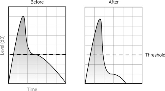
Figure 17.35 Adding punch to a snare using a compressor. The attack is set long enough to retain the natural attack, while the release is set long so gain reduction brings down the natural decay.
We can use exactly the same principle to accent the natural attack, accent transients, revive transients, or reconstruct lost dynamics (due to over-compression, for example). All we need to do is apply some makeup gain after bringing down the decay. Figure 17.36 illustrates this. We can see that after the addition of makeup gain, the attack is emphasized compared with the input signal before compression.
There is more in the dynamics reshaping examples above than first meets the eye. Compression is a sophisticated way of bringing instruments forward or backward in the mix. Perhaps we want to bring the kick forward, but raising the fader detaches it from the mix and makes it too dominant. On the same basis, we might want to pull the kick back a bit, but even gentle lowering of the fader results in a faint kick. One of the problems with using faders is that they affect the full frequency spectrum of sounds. Consequently, this affects the frequency balance of the mix and the masking interaction between instruments. If we want the kick forward in the mix, why not just bring up its attack? If we want it farther away, why not just soften its attack or perhaps its decay? Only affecting a part of the dynamic envelope means we do not have to consider issues such as masking as much. Earlier, we saw how equalizers can provide a surgical alternative to faders by only affecting limited frequency ranges in sounds. Compressors (and other dynamic range processors) can achieve something similar, except they affect limited time (or length) of sounds. In essence, compressors can be used for sophisticated level adjustments as a kind of surgical faders.

Figure 17.36 Accenting the attack of a snare using a compressor. The attack is set long enough to retain the natural attack, while the long release brings down the decay. After applying makeup gain, the attack is made louder, but the decay returns to its original level.
Compression can be used to bring instruments forward and backward in the mix.
![]()
Track 17.65: Reshaping Source
The source drums used in the following samples. The snare in this track is not compressed.
Track 17.66: Reshaping More Attack
For the purpose of demonstration, the attack of the snare is accented to an exaggerated degree. First, the ratio was set to the maximum of 100:1, both time constants were set to minimum, and the threshold was brought down to –40 dB. Then the attack was lengthened, and the longer it became, the more of the natural snare attack passed through; it ended up at the maximum value of 300 ms. (This extremely long attack was required due to the extreme gain reduction of around 15 dB. There are less than 200 ms between the first and second hit, but remember that the attack time determines the rate—not the time—it takes gain reduction to rise.) The release was then lengthened to 1 second so as to track the natural snare decay. The gain reduction was set to +11 dB in order to bring the snare decay back to its original level. Notice how the snare has more punch now, and how it has moved forward in the mix. Also, notice that, as opposed to the previous track, the attack of each hit is not consistent in level. This is due to the release not recovering fast enough between the hits. The sooner each consecutive hit arrives, the less attack it has. For example, the first hit has the loudest attack, and the one straight after it has the softest. There is little we can do about this since shorter release means that the decay of the snare would alter; either bringing the threshold or the ratio down in order to reduce the amount of gain reduction (and thus the quicker the gain would recover) would mean less natural attack compared to decay. We will soon see how this can be resolved using another compressor.
Track 17.67: Reshaping Less Attack
The settings involved in reducing the attack of the snare are completely different from the ones used in the previous track. This time, we only want the compressor to reduce the natural attack without affecting the decay. The threshold is set to –13 dB, a level above which the snare only overshoots by 5 dB. The ratio is set to 3.2:1. Both the attack and release are set to minimum –14 µs and 5 ms, respectively. No makeup gain is applied. The result of this compression is a snare with less punch, positioned farther back in the depth field.
Track 17.68: Reshaping Reviving Attack
For the sake of demonstrating how a compressor can revive lost transients, the attack-lacking snare from the previous track is fed through another compressor with the same settings as in Track 17.66. It is hard to miss how it has regained some healthy attack.
Plugin: Digidesign DigiRack Compressor/Limiter Dyn 3
Drum: Toontrack EZdrummer
One case we have not touched upon yet is how compression can be used to emphasize decay. Although compression brings levels down, we have already seen how we can accent the natural attack by attenuating the decay then raising the makeup gain. To emphasize decay, we attenuate the attack but leave the decay as is, then the makeup gain brings the whole signal up. This can be extremely useful when we want reverbs to be more present. The compressor settings in this case involve low threshold, high ratio, fast attack, and fast release so the gain reduction recovers as quickly as possible. Figure 17.37 illustrates this. The very same settings can be used to lengthen the sustain of instruments, notably guitars. It should be noted, however, that compressing natural reverbs is known to impair the spatial information within them—a faithful sense of space is dependent on the reverb’s natural dynamics (notably its decay). If reverbs are to appear natural, extra care has to be taken while compressing them. Conversely, when reverbs are used in a creative context, compression can easily improve the effect.
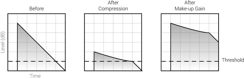
Figure 17.37 Emphasizing the decay of a reverb. The low threshold, high ratio, and fast attack reduce the reverb quickly and drastically. As the reverb decays, the gain reduction recovers quickly due to quick release settings. After applying makeup gain, the reverb decay becomes evidently louder.
While percussive instruments are a good source for demonstrating the attack and release controls, we should not forget that microdynamics control can also be useful for less percussive instruments. Taking an acoustic guitar as an example, sometimes its sound is too jumpy due to, say, the use of a small diaphragm condenser microphone. This is not in the sense that it fluctuates in levels; it might simply sound “liver than life.” We can use a compressor to smooth spiky microdynamics and make the overall sound more rounded.
De-essing
One way to treat sibilance is to attenuate the voice whenever sibilance occurs. This is done by feeding into the side-chain a signal that rises significantly in level whenever sibilance occurs. To achieve this, we boost the sibilance frequency on the side-chain signal, while often also filtering frequencies below it. Whenever the sibilance peaks, the side-chain signal overshoots the threshold and the compressor pulls down the overall voice. One issue with this manual approach is that it attenuates not only the sibilance, but the rest of the voice as well, including its body and higher harmonics. Another issue is that the sibilance on low-level passages might not be loud enough to overshoot the threshold, so only the sibilance on loud passages is treated. A well-designed dedicated de-esser takes into account these two issues, so it is most likely to do a better job.
Making programmed music sound more natural
The dynamic complexity of real performance is beyond comparison to what any computer can simulate. To give an example, synthesizers have attack and release controls, but none of them affect a chord already being played. On a real piano, the sound of every chord alters and is being altered by the chord succeeding it. Another example would be a crash hit—a resting crash being hit would sound different from a hit on a crash already swinging. Snares and many other instruments behave very much the same way. If a programmed musical event is a note, chord, or drum hit, the dynamics of a programmed sequence are applied on each event at a time, but there is no dynamic link between the different events. Compression works on all events as a whole; thus, it can be used to link them in a reallife fashion.
A classic example would be the machine-gun-like sound of programmed snare rolls. Such mechanical arrangements cause each hit to stand out as an individual hit. We can blur the gaps between the hits and meld them together using a compressor. Generally, we want fast attack to make each hit stand out less, and fast release so the decay is retained.
Applying dynamic movement
We have discussed how useful compressors can be for balancing the varying levels of a performance. Unless used to reshape dynamic envelopes, compressors are often associated with the restriction of dynamics. But it is not a secret that a mix with static dynamics can be quite boring. Compressors can be used to get in some action.
To give an extreme example, we can consider an organ playing harmony. The keyboard player changes a chord each bar and all the chords are at reasonably the same level. We can feed this organ into a compressor and feed the kick into the side-chain, and then set low threshold, moderate ratio, fast attack, and a release that will cause full gain recovery by the time the next kick hits. Every time the kick hits, the compressor will attenuate the organ, which will then rise in level until the next kick arrives. It is automatic automation. By attenuating the organ with every kick hit, we also clear some frequency space for the kick. We can also do something similar in order to create more sophisticated drum loops. We can go even further by adding synced delay to an external side-chain signal, so the dynamic movement is triggered by one event, then locks to the tempo.
A compressor as a ducker
A compressor used in the way described above—to attenuate a signal in relation to another signal—behaves like a ducker. A compressor is not really a ducker as the amount of attenuation a compressor applies is dependent on the overshoot amount, whereas a ducker applies a fixed amount. With a compressor, the attenuated signal fluctuates in level in relation to the side-chain signal, which is not the case with duckers. Figure 20.5 illustrates these differences. Percussive instruments are generally less of an issue, since they do not tend to fluctuate as much above the threshold. Also, we can always lengthen the release to slow down gain-reduction changes, but this might not yield musical results once the side-chain signal drops below the threshold. Although for steady ducking it is best to use a ducker, compressors can be, and are, employed as well.
A full exploration of the fascinating ducking applications is presented in Chapter 21. For now, let’s look at a small trick that can turn any compressor into a real ducker. We are trying to prevent the gain reduction from fluctuating in relation to the input signal. We could use long hold or release times, but we need these to control the gain recovery once the side-chain signal drops below the threshold.

Figure 17.38 Making a compressor behave like a ducker. The vocal track is sent to a bus called Gate SC. The moderate track has a signal generator on its first insert slot (generating pink noise), followed by a gate that has its side-chain input set to the Gate SC bus. This moderate track is not mixed, but routed to a bus called Gated Noise instead. On the distorted guitar track, a compressor is loaded, with its side-chain set to the Gated Noise bus.
We have to employ a moderate track. Say we want the vocal to duck the guitars. The moderate track is fed with pink noise, which is gated in relation to the vocal track. We set the gate to open every time the vocal crosses a specific threshold. The moderate track is not mixed to the main mix, but instead routed to the side-chain of the compressor on the guitar track. When the vocal overshoots, the gate opens and the pink noise will trigger the compression of the guitar. The pink noise can be regarded as steady in level, so the guitars will always be attenuated by the same amount. Figure 17.38 shows a snapshot of this setup.
Tricks
Parallel compression
Parallel compression is one of the oldest and more common tricks in mixing. Parallel compression had already been implemented as part of the Dolby A noise reduction system, which was introduced in 1965. In 1977, Mike Bevelle published an article in Studio Sound magazine, which gave this technique much of its publicity. Bob Katz coined the term parallel compression, with other names being side-chain compression (which is confusing since it is not the compressor side-chain we are compressing) and the NY compression trick (NY engineers were notorious for using this technique). It is usually applied on drums, bass, and vocals, although it can be applied on virtually any instrument.
The compression we have discussed so far in this chapter is downward compression— loud signals are brought down in level. One fundamental problem with this practice is that our ears are more sensitive to the bringing down of loud signals than they are to soft signals being brought up. Also, the compression artifacts tend to be more noticeable as they are triggered by loud level signals.
The idea of parallel compression is quite simple—instead of bringing high levels down, we bring the quiet levels up. The ear finds this all the more natural, and the artifacts triggered by low-level signals make the compression effect less evident. In addition, parallel compression retains dynamics much better than downward compression as transients are not brought down—if anything, their bottom is beefed up. Being more transparent, parallel compression lets us drive the compressor even harder when we are after a stronger effect. Also, we can adjust the degree of impact using a single fader rather than a multitude of compressor controls.
Parallel compression lets us make sounds even bigger while retaining their dynamics.
Parallel compression involves a simple setup: take a copy of a signal, compress it, and blend the compressed version with the uncompressed original (Figure 17.39). Generally speaking, the original remains consistent in level and the compressed version is layered below it at a level of our choice.
There are various ways to achieve that within an audio sequencer. If it is a single track in question, we can simply duplicate the track and compress the duplicate. However, if we change something on the original track (e.g., the EQ), we also have to change the duplicate. A more popular approach involves sending the track in question—or a group of tracks—to a bus; the bus is fed into two auxes, and a compressor is only loaded onto one aux (Figure 17.40). We then alter the level of the compressed aux track. We must make sure that there is no delay between the original and the compressed versions or comb filtering will occur—auto delay compensation ensures this will not happen.
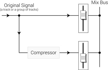
Figure 17.39 Parallel compression is a blend between a compressed and an uncompressed version of the same source. The level of the compressed version is what we alter for more or less effect.
Figure 17.40 Parallel compression in Digital Performer. The output of various drum tracks is routed to a bus called “drumix.” The bus feeds two auxiliaries— drumix and drumix PC. On the latter, a compressor is loaded, and it is blended lower in level with the drumix auxiliary.
While additional routing is required when parallel compression is done on an analog desk, at least one aux track in an audio sequencer could be spared if compressor plugins were given the ability to mix the compressed and the uncompressed input signals (something very similar to the standard wet/dry control on a reverb emulator). While this requires very little effort to implement, only a few compressors provide such a control. The PSP Vintage Warmer 2 in Figure 17.41 is one of them.

Figure 17.41 The PSP Vintage Warmer 2. The Mix control (to the right of the Brick Wall switch) lets us blend the unprocessed input with the compressed version, making parallel compression a very easy affair.
Parallel compression is a form of upward compression—instead of making louder sounds quieter (downward compression), we make quiet sounds louder. But parallel compression is different from upward compression in that low-level signals are boosted in a linear fashion (1:1 ratio), the most drastic ratio happens right above the knee, and from there up the ratio curve slowly returns to 1:1. Figure 17.42 illustrates this. We can consider parallel compression as having the most effect on medium-level signals as they cross the threshold. In practice, however, the threshold is set quite low below the action range, so it is eventually the quiet signals that get most of the effect. In essence, the quieter the signal is, the more it is brought up in level; high-level signals are hardly boosted. This can be very useful for level balancing.
We can see from Figure 17.42a that the ratio transition around the knee can be quite drastic. We can achieve a softer transition in two ways: either bring down the ratio or bring down the level of the compressed version. As we bring down the compressed version in level, the resultant sum will morph toward the unity gain curve of the uncompressed version. With the compressed version all the way down, the resultant sum is identical to the uncompressed version.
The attack time of the compressor is set to be as fast as possible, so sharp transients are not overemphasized (unless this is what we want). If transparency is what we are after, the release time is set to minimize pumping and low-frequency distortion. However, a powerful effect can be achieved if the compressed version is pumping and distorting, and, again, we control how much of this effect blends in using the level of the compressed version.
The parallel compression technique is almost matchless when applied to a group of instruments that has already been dynamically treated, such as a drum mix. Applying a standard compression on a drum mix can easily impair the dynamics of each source track. For example, while setting the drum mix compression, we have to find the right attack and release times that will retain the dynamic character of each drum. Parallel compression makes the whole affair of adding power less restricting.
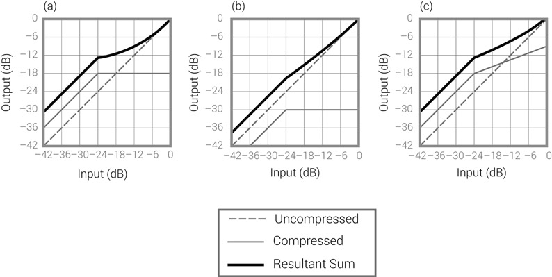
Figure 17.42 Parallel compression and resultant ratio curves. (a) The compressed version, with 1,000:1 ratio, is 6 dB louder than the uncompressed version in order to demonstrate the shape of the resultant ratio curve. We can see that, from the 1:1 ratio below the threshold point, the ratio slowly returns to 1:1 as the signal gets louder. (b) The same settings as in (a), only with a compressed version that is 6 dB below the uncompressed version. We can see a smoother ratio curve above the knee. (c) The same settings as in (a), only with 2:1 ratio. Again, we can see a smoother ratio curve above the knee.
Parallel compression is also one of the rare techniques where a compressor might be used in an aux send arrangement rather than the standard inserts. Taking a drum mix, for example, we can create an alternative submix using sends and feed the send-bus to the parallel compressor. Then, if we want a bit more weight on the kick, the kick send-level is brought up.
![]()
Track 17.69: PC Drums Uncompressed Layer
The uncompressed version of the drums.
Track 17.70: PC Drums Compressed Layer
The compressed version of the drums in the previous track. The compressor is set for heavy effect with the fastest time constants.
The following tracks are simply a blend of the two previous tracks. The uncompressed layer is always mixed at the same level, with the compressed layer always a few dB below it (denoted in each track name). Notice how much better the attack and dynamics are retained compared to standard compression:
- Track 17.71: PC Drums 21 dB down
- Track 17.72: PC Drums 15 dB down Track 17.73: PC Drums 9 dB down
- Track 17.74: PC Drums 3B down
The same set of tracks, but this time involving a bass:
- Track 17.75: PC Bass Uncompressed Layer
- Track 17.76: PC Bass Compressed Layer
The intentional distortion on this track is the outcome of fast time constants.
- Track 17.77: PC Bass 21 dB down
- Track 17.78: PC Bass 15 dB down
- Track 17.79: PC Bass 9 dB down
- Track 17.80: PC Bass 3 dB down
Plugin: Universal Audio Fairchild
Drums: Toontrack EZdrummer
Serial compression
Serial compression, or multi-stage compression as it is sometimes called, is also an old technique. It involves connecting two (or more) compressors in series. In an analog studio, this calls for extra routing and the loss of either a channel strip or an external unit. There is no such overhead with audio sequencers—setting up serial compression simply involves loading two plugins in consecutive insert slots.
The idea behind serial compression is this: If we have two tasks to achieve, why not distribute each task to a different compressor and have the settings on each compressor optimal for its task? For example, if we want to add punch to a snare, but not all the snare hits are at the same level, we can use the first compressor to balance the level of the performance and the second to add punch. This mix-and-match approach is also beneficial since some compressors are better for specific tasks—one compressor might be better at balancing, another at adding punch.
![]()
Track 17.81: Reshaping Balancing Attack
You probably remember the problem in Track 17.66, where the attack of the different hits varied in relation to hit spacing. To solve this, another compressor is inserted following the compressor that accented the attack. The balancing compressor has its threshold set at –18.3 dB, a ratio of 2.8:1, soft-knee, 15 ms attack, 5 ms release, and 3.2 dB of makeup gain.
Plugin: Digidesign DigiRack Compressor/Limiter Dyn 3
Drums: Toontrack Ezdrummer
More on compressors
Compressors, depth, and focus
We have seen in the previous sections how manipulation of the dynamic envelope of instruments can send them backwards or forward in the depth field. Part of this phenomenon has to do with an increase or decrease in the overall level of the treated instrument. There is another important aspect of compression that links it to depth and focus. It involves recordings that include ambiance or reverb.
The relationship between reverbs, depth, and focus will be expounded in Chapter 24 (on reverbs). For now, it is sufficient to say that the more reverb there is compared with the dry sound, the farther away and the less focused sounds will appear. Compression can either increase or decrease the level of a reverb already printed on a recording. It is easy to demonstrate this with a drum recording that contains ambiance, such as overheads or a drum mix. If the compressor is set for short attack and release, the reverb will become louder, making the drums appear farther back and their imagemore smeared. If the compressor is set with an attack long enough to let the natural attack through, and longer release so some gain reduction is still applied on the ambiance in between hits, the drums will appear closer and their image will sharpen.
![]()
Experienced or attentive readers have probably noticed the effect of compression on depth and focus in virtually all previous samples that included a drum kit. For example, in Track 17.2, the drums move farther back as the threshold drops. Here are three more tracks demonstrating this.
Track 17.82: Drums III Uncompressed
The source track to be compressed in the following two tracks.
Track 17.83: Drums III Backwards
Short time constants and gain reduction peaking at around 7 dB are enough to noticeably increase the ratio of the ambiance level. This sends the drums backward in the depth field and makes their image less focused.
Track 17.84: Drums III Forwards
The long attack and moderate release in this track are set to let the kick and snare pass through but maintain some gain reduction after each hit, thus reducing the level of the ambiance. Both drums appear more frontal and focused.
Plugin: Sonnox Oxford Dynamics
Drums: Toontrack Ezdrummer
Setting up a compressor
There are various ways to tackle the initial settings of a compressor. The method mentioned here provides a step-by-step approach that can be helpful in many situations, notably when compressing vocals or drums. People new to compression are the most likely to find this technique useful. It can also be used as an aural exercise—it makes the function of each control appear rather obvious. This method is based on three main stages— the extent, degree, and timing—which in relation to controls are threshold, ratio, and attack and release.
- Initial settings—the idea is to have the most obvious compression once the threshold is brought down in the next step. All controls but the threshold are set to produce the hardest possible compression.
- Threshold all the way up (so no compression takes place initially).
- Ratio all the way up.
- Attack and release as short as possible.
- If there is any option regarding peak/RMS or soft-/hard-knee, these are better set at this point based on the nature of the instrument. For the purpose of the aural exercise, peak and hard-knee are preferred.
- Determine extent—threshold goes down. Due to all the other settings, as soon as signals overshoot, the compression becomes very obvious and on many compressors the fast attack and release will cause audible distortion. We can easily identify what portion of the signal is being compressed and adjust the threshold accordingly. It can be beneficial to set the threshold slightly below what seems to be the appropriate setting, as later it can lead to more uniform compression.
- Determine degree—ratio goes down from maximum. Once we know the extent of compression, we can determine its degree.
- Determine attack—the attack is made longer from its initial short settings.
- Determine release—the release is also made longer.
There is a sense to the order in which controls are set with this method. Changes to the threshold and ratio will cause changes to the amount of gain reduction, which in turn affect the overall attack and release times (the more gain reduction, the slower the attack and release). So the attack and release are set after the threshold and ratio. The attack is set before the release, since long release settings might interfere with succeeding attack phases. While this method can get very close to what we need, usually fine-tuning each control will follow.
![]()
Here is a demonstration of the steps involved in this method, using the uncompressed vocal in Track 17.17. The compressor is initialized as described above, and to make the effect more obvious the knee is set to hard.
Track 17.85: Vocal Steps Threshold
The threshold was brought down, ending at –22 dB. This level is slightly lower than what might seem to be needed, to allow longer attack later on.
Track 17.86: Vocal Steps Ratio
The ratio is brought down from 1,000:1 to 3:1, at which the vocal is reasonably balanced.
Track 17.87: Vocal Steps Attack
One problem with the previous track is that the function of the attack was too obvious, so it has been lengthened to 1.85 ms. The release is left untouched at the minimum value of 5 ms.
Plugin: Sonnox Oxford Dynamics
Multiband compression
The compressor we have discussed so far is known as a broadband compressor—it attenuates the whole input signal, with its full frequency spectrum. We have already seen some issues this can bring about—it can cause the dulling of sounds due to high-frequency attenuation when low frequencies trigger the compression. Also, when we compress a bass guitar, low notes will result in more gain reduction, which also affects the mid and high frequencies that give the bass guitar much of its definition. When we de-ess vocals, we attenuate not only the sibilance, but also the body and the higher harmonics of the voice.
A multiband compressor, or a split-band compressor, splits the input signal into different bands, then lets us compress each band individually (Figure 17.43). For example, for de-essing we can define a band between 3 and 8 kHz, and only sibilant peaks at this frequency range will be compressed, without affecting the rest of the frequency spectrum. We can employ the same principle when trying to de-emphasize the resonance of an acoustic guitar.
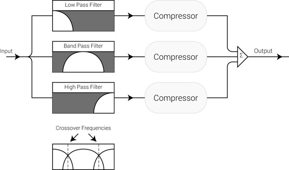
Figure 17.43 A block diagram of a multiband compressor. In this illustration, a three-band compressor is shown. The input signal is split into three, and filters are used to retain the respective frequencies of each band. Then each band is treated with its own compressor, and the three bands are summed together to constitute the output signal. At the bottom, we can see the combined effect of the filters and the crossover frequencies between the different bands.
The manufacturing of an analog multiband compressor is more costly as it involves more than one compressor and a quality crossover. While being a standard tool in mastering studios, multiband compressors were never high up in the mixing priority list. However, software plugins cost nothing to manufacture, so these have made multiband compressors more widespread today (Figure 17.44).
Most multiband compressors have a predefined number of bands and they let us set the crossover frequencies between the different bands. A dedicated compressor per band should offer most related controls. Some controls might still be global and affect all bands.

Figure 17.44 The Universal Audio Precision Multiband. This plugin offers a compressor, expander, or a gate for each of the five bands. On the left are the controls for the compressor of the selected LF. The plot in the middle shows the frequency division between the five bands. The meters on the right show the gain reduction per band.
Multiband compressors provide great advantages when the signal in question is of a broadband nature, such as a stereo mix. Compressing each band individually provides a greater degree of control over the signal. This is why multiband compressors are so popular in mastering. Nevertheless, every instrument being mixed can be divided into a few separate frequency bands that each play a different role, and we can benefit from compressing each band individually rather than the instrument as a whole; for example, the lows of a kick and the attack on its high-mids. The softer the drummer hits the kick, the less are the lows compared with the click of the beater. We can compress the low band while compensating with some makeup gain specifically on that band. This will make the lows-to-attack ratio more consistent with different hit velocities. We can apply the same principle on a bass guitar in order to achieve more solid frequency balance for different notes. We can also reverse this idea in order to make a programmed kick more natural. Unless velocity layers are used, kick samples have the same ratio between lows and high-mids. We can set a low threshold and a low ratio on the high-mid band, so the higher the hit velocity is, the more the high-mid attack will be compressed. This will alter the ratio between the lows and attack like in the real world. Last but not least, multiband compression is an excellent way to rectify the proximity effect on vocal tracks–the low-end boost resulting from the vocalist moving closer to the microphone. Compressing the low bands rectifies these variations.
Another advantage of using multiband compressors is that, while only affecting a specific frequency band, they tend to interfere less with the overall tonality of the processed signal. In addition, the compression on each band can be pushed harder since the compression artifacts are introduced on a limited range of frequencies. For example, fast release on the lower band will cause distortion, but we can dial a faster release on the higher bands, which will make these bands louder. By making each band louder separately, we can make signals even louder than we could with a broadband compressor. It is a divide and conquer approach applied to the frequency domain. Although they involve more effort and time to set (and a little more auditory skill), multiband compressors give us more control over the dynamic treatment of sound.
When a multiband compressor is not available, we can set up a manual arrangement using an array of filters and broadband compressors. Say we need two bands, we can send a track to a bus and bring the bus back into two different tracks, put a low-pass filter on one and a high-pass filter on the other, then set both to the same cut-off frequency. Next, we insert a compressor on each track, and send both at the same level to the mix bus. Were multiband compressors as simple as explained so far, this manual setup would work flawlessly. However, multiband compressors involve some additional science in the way they sum the different bands back together. For example, they might align the phase of the different bands. Manual multiband compression does work, but a true multiband compressor should sound better.
![]()
Track 17.88: Bass Multiband
This track demonstrates how a multiband compressor can be utilized to reduce squeaks. In the original bass recording (Track 17.38), there are two noticeable nail squeaks on the A/G# notes, and then a few more toward the end. Squeaks as such might be masked when the guitar is mixed with other instruments, but they can become annoyingly noticeable if the bass is equalized, distorted or processed using an enhancer. The compressor is set with a single active band between 444 Hz and 3.3 kHz. Heavy gain reduction occurs on this band only when the squeaks happen. Compare this track to the original to see the difference.
Track 17.89: Bass Multiband SC
Most multiband compressors let us solo each band. This is the soloed version of the active band in the previous track, with its compressor disabled. Essentially, this signal feeds the side-chain of the compressor on the band used.
Plugin: Universal Audio Precision Multiband
Before or after the EQ?
What seems like an eternal mixing question is: Should a compressor come before or after an equalizer? Had there been a determined answer, this question would not be asked. The answer is: it depends. Let’s see on what.
We have already established that low frequencies excite compressors more than high frequencies. There are additional situations where we clearly do not want the compressor to respond to a specific frequency range of the input signal, in which case an equalizer has to be placed before the compressor. For example, we might want to filter the lows of vocals or overheads before compressing them. The problem with a pre-compressor equalization is that any changes to the equalizer affect the characteristics of the compression. So, once the compressor is set, touching the equalizer might require a revisit to the compression settings.
So the wisdom is this: for compression-related equalization, we should put an equalizer before the compressor. Any other equalization should be done after the compressor. This includes equalization that alters the tonality of an instrument or one that compensates for the tonal alterations caused by the compressor.
All but compression-related equalization should be done after the compressor.
Many compressors nowadays let us equalize the side-chain signal. When such a facility exists, equalizers are most likely to be placed after the compressor. There is a huge benefit of using side-chain equalization rather than pre-compressor equalizers. With pre-compressor equalizers, the tonality of the signal is affected by two equalizers—the one before and the one after the compressor. However, the pre-compressor equalizer is said to be locked for the reasons explained above. None of this happens with side-chain equalization—the tonality of the signal is solely controlled by a single equalizer placed after the compressor. Perhaps the only shortfall of using side-chain equalizers is that they often provide fewer bands, or less control, than a standard equalizer. These might not be sufficient for our needs, so pre-compressor equalizers might still be employed.
Providing their facilities are adapted for the task, side-chain equalizers provide great benefit over pre-compressor equalizers.
Having said that, it pays to remember that post-compressor equalizers can damage the dynamic control achieved by the compressor. For instance, we might have balanced vocals out of the compressor, but then boosting around 1,760 Hz would make all the A notes jump out (1,760 Hz is A, and thus a harmonic of all A notes below it). There is no magic solution to such a problem. Sometimes the choice of pre- or post-compressor equalizer is a matter of experimentation.
Compressors on the mix bus
Engaging a compressor on the mix bus while mixing, also known as bus compression, is another source of a long debate in the mixing community. Some mixing engineers use bus compression passionately from very early stages of the mix. Often they have at their disposal a respectable compressor, such as the SSL bus (or quad) compressor, and they drive it with rather subtle settings. The bus compressor might be used during the majority of the mix, but it is often switched out before the mix is printed—mastering engineers seem rather united against mixes that have already been stereo-compressed. Conversely, some mixing engineers would rather be mixing on the edge of an airport runway than mix with a compressor on the mix bus—they are that much against it. Both types include some of the world’s most creditable mixing engineers.
Perhaps the least practical reason for using bus compression is that it simply makes the mix more exciting, and excitement is an important part of mixing. Bus compression also lets us evaluate how the mix might translate to radio or in clubs—both involve heavy compression and/or limiting in their signal chain. Mostly in these situations, we care how the low-end affects the rest of the mix. Is the kick too boomy? Is it thin?
There are a few risks in using bus compression. The greatest of them is that it limits our ability to judge relative levels. If the bus compressor is set to anything but subtle, it should be no wonder if, when it is bypassed, the mix relative levels turn chaotic. Also, by applying compression, signals that overshoot the threshold are reduced by a specific ratio. If a fader is brought up by 4 dB, its instrument might only raise by 1 dB due to a 4:1 ratio on the bus compressor. In the way compressors work, pushing the kick up might result in more compression of low frequencies, which can actually make the kick quieter (there is no individual makeup gain when the stereo mix is compressed). So it is not only the precision of the faders that we can lose with bus compression—level changes might be opposite to fader movements. Another thing to ask is how exactly one should go about servicing the bus compression. Any change in the mix can also affect the compression. So should we revisit the bus compressor after every mixing move? It should be clear that only respectable compressors and subtle settings would be fit for the task.
Perhaps above all comes the idea that only trained ears can recognize the subtleties of bus compression. For the novice, bus compression can be like a translucent layer that only blurs what is behind it—the actual mix.
Unless you have a good compressor, subtle settings, and trained ears, bus compression can be self-defeating.
Dynamic convolution compressors
The concept of convolution, in simple terms at least, involves capturing the characteristics of a specific audio system so they can be emulated digitally. The remarkable thing about this process is that it is done without any knowledge of how the system actually works— it simply involves learning the system response (output) to input signals. While the concept might seem rather complex, it is a truly simple one—we can take a vintage analog unit, learn its characteristics, then build a plugin that emulates these characteristics. If all the science is done properly, the plugin will sound very much like the original unit.

Figure 17.45 The Focusrite Liquid Mix.
Convolution reverbs are now widely known and will be discussed in Chapter 24. Dynamic convolution is a fairly new technology, developed by a company called Sintefex Audio. Dynamic convolution is far more complex than the convolution process of reverbs. In order to learn the characteristics of compressors (or equalizers), a tedious series of measurements has to be taken before any simulation can be crystallized. Theoretically, it involves studying the compressor response to any possible combination of input levels, frequencies, and settings on the unit itself. In practice, not every possible combination is studied, but a large-scale step-wise approach is taken instead. For example, instead of studying every possible ratio setting, we might only learn integer-based ratios (1:1, 2:1, 3:1, 4:1, 5:1, and so forth). In theory, the emulating processor would only offer the settings that were studied —if only integer-based ratios were learned, the emulator would not offer a 2.5:1 ratio. This could be an annoying limitation. Luckily, the current technology allows dynamic convolution compressors to offer settings that were not studied, and smart algorithms produce an approximate result (a 2.5:1 ratio would produce something between 2:1 and 3:1).
Dynamic convolution is mostly known for its usage in the Focusrite Liquid Channel and Liquid Mix. The former is a hardware unit, the latter is a DSP platform for DAWs. The Liquid Mix, shown in Figure 17.45, includes emulations of 40 compressors (and 20 equalizers) that pretty much constitute a list of the most respectable units one can find in a professional studio.