Delay time

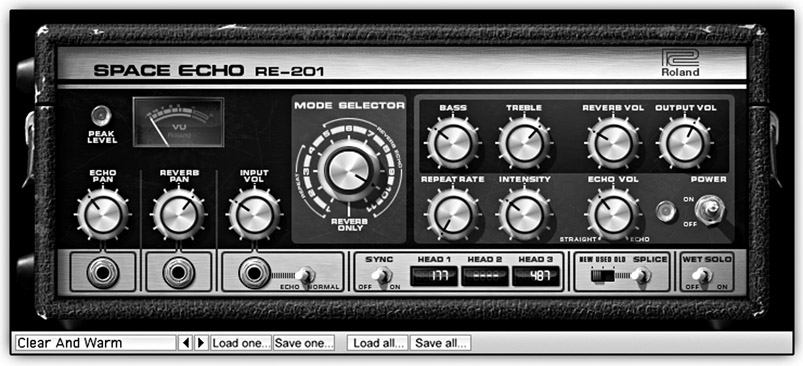
Figure 22.1 The Universal Audio Roland RE-201 Space Echo. This plugin for the UAD platform emulates the sound of the vintage tape loop machine. The interface looks very similar to that of the original unit.

The most basic requirement of a delay unit is to delay the input signal by a set amount of time. This can be achieved using the basic arrangement shown in Figure 22.2. A magnetic tape loop rolls within the unit, where a device called a capstan controls its speed. The tape passes through three heads: the erase head, the record head, and the playback head (also known as the replay head). After previous content has been erased by the erase head, the input signal is recorded via the record head. Then it takes a period of time for the recorded material to travel to the replay head, which feeds the output of the unit. The time it takes the tape to travel from the record to the replay head determines the delay time.

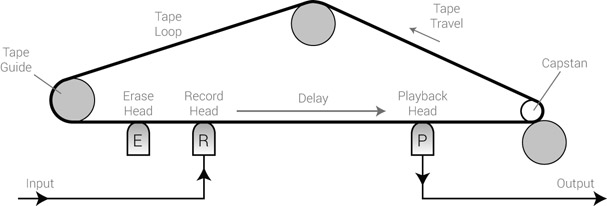
Figure 22.2 Simple tape loop.

There are two ways to control the delay time: either changing the distance between the record and replay head or changing the tape speed. Moving any head is a mechanical challenge, and it is much easier to change the tape speed. There is a limitation, however, to how slowly the tape can travel, so some units employ a number of replay heads at different distances, and the rough selection of delay time is made by selecting which head feeds the output. The tape speed is then used for fine adjustments.

Modulating the delay time

The delay time can be modulated—shortened and lengthened in a cyclic fashion. For example, within each cycle, a nominal delay time of 100 ms might shift to 90 ms, then back to 100 ms, then to 110 ms, and back to the starting point—100 ms. This pattern will repeat in each cycle. How quickly a cycle is completed is determined by the modulation rate (or modulation speed). How far below and above the nominal value the delay time reaches is known as the modulation depth.

If heads could easily be moved, modulating the delay time would involve moving the replay head closer to or farther away from the record head. But since it is mostly the tape speed that grants the delay time, a special circuit slows down and speeds up the capstan. There is an important effect to this varying tape speed—just as the pitch drops as we slow a vinyl, the delayed signal drops in pitch as the capstan slows down; and similarly, as the capstan speeds up, the delayed signal rises in pitch. These changes in pitch are highly noticeable with both high modulation-rate and depth settings.

Feedback

Using the arrangement discussed so far, with no feedback applied, the delayed copy would produce a signal echo when mixed with the original signal. It is often our aim to produce repeating echoes, whether in order to simulate the reflections in large spaces or as a creative effect. There is a very easy way to achieve this, which simply involves routing the replay signal back to the record head (Figure 22.3). This creates a feedback loop where each delayed echo returns to the record head, then is delayed again. Providing a fixed delay time of 100 ms, the echo pattern will involve echoes at 100, 200, 300, 400, 500 ms, and so forth.

A feedback control determines the amount of attenuation (or sometimes even boost) applied on repeating echoes. If this control attenuates, say by 6 dB, each echo will be 6 dB quieter than its preceding echo, and the echoes will diminish over time. If the feedback control is set to 0 dB or higher, the echoes will become progressively louder until the tape saturates (even 0 dB produces such an effect as either tape hiss or the input signal cause increasing level when mixed with the echoes). Such rising echoes are used as an effect, but at some point the feedback has to be pulled back to attenuation or the echoes will continue forever, causing increasingly distorted sound.

You probably noticed the phase switch before the feedback level control. This switch inverts the phase of the signal passing through the feedback loop (on some units, this is achieved using negative feedback). The first echo is phase-inverted compared with the input signal.

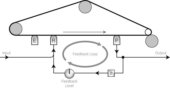
Figure 22.3 Tape delay with feedback loop.

But once this echo is delayed again and travels through the loop as the second echo, its phase is inverted again to make it in-phase with the input signal. Essentially, the phase flips per echo, so odd echoes are always phase-inverted compared with the input signal, while even echoes are in-phase. Very short delay times cause comb filtering and can alter the harmonic content of the material quite noticeably. Inverting the phase of signals traveling through the feedback loop alters this comb-filtering interaction—sometimes for the better, sometimes for the worse.

Wet/dry mix and input/output level controls

Like most other effects, most delays let us set the ratio between the wet and dry signals. There might also be input and output level controls. Figure 22.4 incorporates these controls and shows the final layout of our imaginary tape-echo machine.

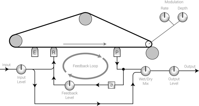
Figure 22.4 A tape-echo machine with all common controls.

The tape as a filter

Tapes do not have a flat frequency response. This is one of the most important characteristics that distinguish them from precise digital media, for recordings in general, and in relation to delays in particular. The most noticeable aspect of this uneven frequency response is the high-frequency roll-off, which becomes more profound at lower tape speeds. Essentially, a tape can be looked at as having an LPF with its cut-off frequency dependent on the tape speed (and quality). In relation to tape delay, each echo experiences some degree of softening of high frequencies. Repeating echoes become progressively darker, which, in our perception, makes them appear slightly farther away.

The simple delay

The simple delay (Figure 22.5) has a single feature—delay time, which is set in either samples or milliseconds. Often this type of process is used for manual plugin delay compensation, but we will see later that even such a simple delay can be beneficial in a mix.

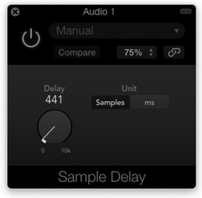
Figure 22.5 A simple delay plugin.

Modulated/feedback delay

Figure 22.6 shows the Digidesign Mod Delay II in its mono form. The plugin offers the standard functionality of a DDL: input gain, wet/dry mix, an LPF, a delay time set in milliseconds, modulation depth and rate, and feedback control. The LPF is placed within the feedback loop to simulate the high-frequency roll-off typical of tapes. In the case of the Mod Delay II, the phase switch simply inverts the input signal phase, not that of the feedback signal.

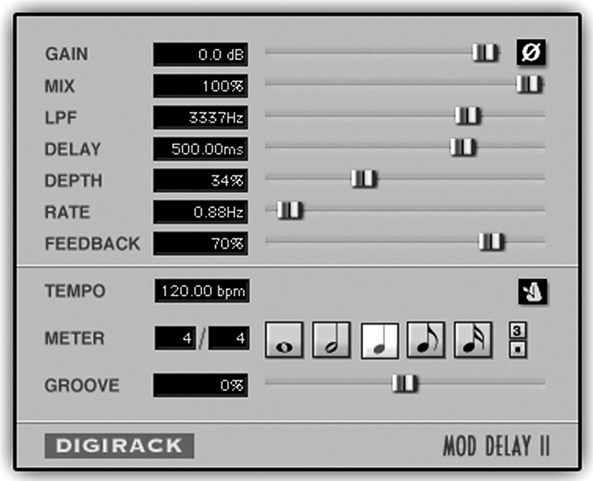
Figure 22.6 The Digidesign DigiRack Mod Delay II.

The depth parameter is often given in a percentage and determines the delay time alternation range. For example, with a delay time of 600 ms, 100% depth denotes 600 ms difference between the shortest and longest delays, which would result in a delay time within the range of 300–900 ms. It is worth mentioning that the higher the delay time, the more effect the depth will have—while 50% depth on 6 ms means 3 ms difference, the same depth on 600 ms would yield 300 ms difference. The modulation rate can be in Hz, but can also be synced to the tempo of the song. There is some link between the modulation depth and rate settings, where the higher the depth is, the slower the rate needs to be for the effect not to sound peculiar.

It is worth noting the tempo-related controls in Figure 22.6, which are a very common part of digital delays. In its core, instead of setting the delay time directly in milliseconds, it is set based on a specific note value. In addition to the common values, such as quarter-notes, there might also be triplets and dotted options. Often a dotted quarter-note will appear as 1/4D, and a half-note triplet will appear as 1/2T. But the truly useful feature of DDLs is their ability to tempo-sync—given a set note duration, the delay time will alter in relation to the changing tempo of the song. This way, as the song slows down, the delay time is lengthened. On a digital delay unit, this often requires MIDI clock-based synchronization. Plugins, on the other hand, natively sync to the changing tempo of the session. In cases where the musicians did not record to a click, a tempo-mapping process can map tempo changes to the tempo ruler.

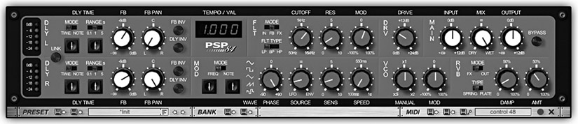
Figure 22.7 The PSP 84.

From the basic features shown in Figure 22.6, delays can involve many more features and controls. One of the more advanced designs—the PSP 84—is shown in Figure 22.7. Among its features are separate left and right delay lines, a modulation source with selectable waveforms and relative left/right modulation phases, a resonant filter of three selectable natures, a drive control to simulate the saturation of analog tapes, and even an integral reverb. In addition, the various building blocks can be configured in a modular fashion typical of synthesizers. For example, the modulation section can affect both the buffer-playback speed and the filter cut-off. The comprehensive features on the PSP 84 make it capable of producing a wider variety of time-based effects than just plain delays. But at least some of these features are often also part of other delay lines.

Ping-pong delay

The term ping-pong delay describes a delay where echoes bounce between the left and right channels. If both channels’ feedback gets sent to the opposite channel, the resultant signal flow would behave the same way as in Figure 22.8.

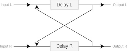
Figure 22.8 A pure ping-pong delay.

Although there are some dedicated ping-pong delays (mostly programs within a unit or a plugin), any stereo delay that lets us pan the feedback from one channel to the other can achieve such behavior. Instead of offering feedback pan control per channel, some plugins offer two controls per channel: feedback and feedback crossfeed to the opposite channel. Such a plugin is shown in Figure 22.9.

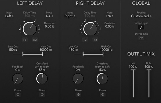
Figure 22.9 The Logic Stereo Delay.

Multitap delay

The feedback mechanism, despite its wide use, has some limitations: the echoes are spaced at regular intervals, their level drops in a predictable way, and their frequency content is correlated. We say that each echo is dependent on the echo preceding it. Sometimes we have a very clear idea of the exact number of echoes we would like, what their level should be, or where they should be panned, and we wish to have full control over their spacing and frequency content. A multitap delay is designed to provide such precise control.

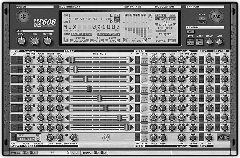
Figure 22.10 The PSP 608 multitap delay.

Converting a standard tape delay into a multitap delay would involve adding, say, seven playback heads (each considered as a tap), giving us the ability to position each within a set distance from the record head and providing a separate output for each head. These are rather challenging requirements for a mechanical device, but there is no problem implementing multitap delays in the digital domain. Figure 22.10 shows the PSP 608 (an eight-tap delay). We have individual control over each echo’s timing (horizontal sliders), gain, pan position, feedback send, and filter.

Phrase sampler mode

This is an added feature on some delay units (also called freeze looping) that enables the sampling of a specific phrase and then playing it over and over again. A unit might provide freeze and trigger switches or a single switch that simply enters the mode by replaying part of the currently stored buffer. Many units can tempo-sync this feature so all sampling and triggering lock to the tempo of the song. This feature is different from setting the feedback to 0 dB, since with phrase samplers each repeat is identical to the original sampled material (whereas in feedback mode each echo is a modified version of the previous echo).

Delay times

Different delay times are perceived differently by our ears and thus play a different role in the mix. We can generalize and say that short delays are used very differently from longer delays. What varies between the two is whether or not we can discern distinct echoes. Yet, we can categorize delay times even further into five main groups. The times shown here are rough and vary depending on the instrument in question:

• 0–20 ms—very short delays of this sort, provided the dry and wet signals are mixed in mono, produce comb filtering and alter the timbre of instruments. Applications for such short delays often involve modulation of the delay time and are discussed in the next chapter. If the dry and wet signals are panned each to a different extreme, the result complies with the Haas effect.
• 20–60 ms—this range of time is often perceived as doubling. However, it is the cheapest-sounding approach to doubling, which can be improved by modulating the delay time.
• 60–100 ms—a delay longer than approximately 60 ms is already perceived by our ears as a distinct echo. Nevertheless, the short time gap between the dry and wet sounds results in what is known as slapback delay—quick, successive echoes, often associated with reflections bouncing between parallel walls. Slapback delays are used (in the past more than today) as a creative effect. Since slapback delay could be easily produced using a tape machine, it was extremely popular before digital delays emerged and can be recognized in many mixes from the 1960s.
• 100 ms quarter-note—such delay times are what most people associate with plain delay or echo, where echoes are spaced apart enough to be easily recognized. For a tempo of 120 bpm at common time, a quarter-note would be 500 ms. Delay times within this range are very common.
• Quarter-note and above—long delay times as such are perceived as grand-canyon echoes.

Panning delays

The delay output can be either mono or stereo. In the case of stereo output, where there is a clear difference between the left and right channels, the echoes are often mirrored around the center of the stereo panorama or around the center position of the source instrument. As an example, if vocals are panned center, the echoes might be panned to 10:00 and 14:00. Mono delays can be panned to the same position as the source instrument, but often engineers pan them to a different position, so they do not clash with the source instrument. This not only makes the echoes more defined, but also widens the stereo image of the source instrument. Very often, if the instrument is panned to one side of the panorama, its echoes will be mirrored on the other side. Instruments panned center will normally benefit from a stereo delay, so the effect can be balanced across the sound stage. But there are quite a few examples of an instrument panned center with its mono delay panned only to one side.

Tempo-sync

It would seem very reasonable to sync the echoes to the tempo of the song, especially in the various dance genres. Since delay is the most distinct timing-related effect, offbeat echoes can clash with the rhythm of the song and yield some timing confusion. Delays longer than a quarter-note are especially prone to such errors.

However, there are situations where it actually makes sense to have the echoes out of sync. First, very short delay times, say those shorter than 100 ms, seldom play a rhythmical role or are perceived as having a strict rhythmical sense. Second, for some instruments, tempo-synced echoes might be masked by other rhythmical instruments. For example, if we delay hi-hats playing eighth-notes and sync the delay time, some of the echoes will overlap with the original hits and be masked. Triplets, three-sixteenth-notes, and other anomalous durations can often prevent these issues while still maintaining some rhythmical sense. Perhaps the advantage of out-of-sync delays is that they attract attention, being contrary to the rhythm of the song. This might work better with occasional delay appearances, where these offbeat echoes create some tension that is later resolved.

It is worth remembering that before audio sequencers became widespread, engineers had to calculate delay times in order to sync to the tempo of the song. Despite the knowledge of how to do this, often delay times were set based on experiment rather than calculations, and, indeed, often the result was not strict note values.

Filters

Echoes identical to the original source can be quite boring. In addition, if these are quite loud compared with the original, they can be mistaken for additional notes rather than echoes. Although the complexity of tape delay is greater than what simple filtering can achieve, the feedback filters let us incorporate some change and movement into the otherwise statically repeating echoes and distinguish them from the original sound. An LPF makes each echo slightly darker than the previous one, which also makes the echoes progressively undefined and distant. An HPF has the opposite effect—it makes each echo more defined, so, despite their decreasing level, late echoes might be perceived better. Yet they will be distinguishable from the original sound.

Modulation

The modulation feature of a delay line is mostly used with very short delay times. This is done in order to enhance effects such as chorusing or create effects such as flanging. It can be used with longer delay times to add some dimension, movement, or size to a simple delay line, but with anything more than subtle settings the change in pitch becomes evident. This might be appropriate in a creative context, but less so in a practical context.

The automated delay line

One very early and still extremely popular mix practice is automating a delay line. Done mostly on vocals or other lead elements, we often want the delay to catch the very last word or note of a musical phrase. To achieve this, we automate the send level to the delay unit, bringing it up before the word we wish to catch, then down again. Depending on the exact effect we are after, the feedback is set to moderate so the echoes diminish over time, or we set it high to create echoes that barely decline, then we cut the effect by turning the feedback all the way down.

Add sense of space and depth

A detailed exploration into our perception of depth is given later in Chapter 24, on reverbs. For now, it is sufficient to say that the very early reflections from nearby walls and other boundaries give our brain much of the information regarding spatial properties and the front/back position of the source instrument in a room. To be frank, reverb emulators are designed to recreate a faithful pattern of such early reflections, and they do so much better than any delay line. However, even the simplest echo pattern caused by a stereo delay can create a vague impression of depth—it is unlikely to sound as natural as what most reverbs produce, but it will still have some effect.

One advantage that delays have over reverbs is that reverbs provide far denser sounds that can consist of thousands of echoes. So many echoes might not only produce an excellent space simulation, but also cloud the mix and cause some masking. Delays, on the other hand, are far more sparse and often only involve a few echoes. When natural simulation is not our prime concern, or in cases where vague space is what we are after, delays may be suitable for the task.

There is another important advantage in the vague simulation that space delays produce— they do not tend to send instruments to the back of the mix as much as reverbs do. This lets us add some sense of space, while still keeping instruments in the front of the mix.

Add life

This use, to some extent, is very similar to the previous one—by adding some echoes to a dry instrument, we add some dimension that makes its sound more realistic. Again, the idea that any depth and distance are vague is often an advantage here. Perhaps the main beneficiary of this type of treatment is the vocals—we can add some vitality and elegance, without sending them backward in the mix.

Natural distance

If we imagine a large live room where all the musicians are positioned in front of a stereo pair, the sound arriving from musicians right at the back would have to travel farther (ergo for a longer time) than the sound arriving from musicians close to the microphones. As sound takes approximately 1 ms to travel 1 ft, the sound from a drummer placed 25 ft (approximately 8 m) from the microphones would take around 25 ms to travel. It would take around 3 ms for the voice to travel from a singer 1 m away. In many recordings done today using overdubs, there is no such delay—apart from the overhead, all other instruments might be recorded with close-mics, often no farther than 2 ft away. Essentially, when all these overdubs are combined, it would create the impression that all the musicians were playing equidistant from the microphone; in other words, the very same line in space. Although it is primarily reverbs that give us the impression of depth, this very sense can be enhanced if we introduce some short delay on instruments we want farther away in the mix. In this specific case, we only mix the delayed signal without the original one and make no use of feedback or modulation.

Fill time gaps

The echoes produced by a delay can fill empty moments in the mix where nothing much develops otherwise. For this task, a generous feedback is often set along with relatively long delay times, and a filter is used to add some variety to the echoes. We usually want the delay to fill a very specific gap and diminish once the song moves on, so this application often involves an automated delay line with ridden feedback.

Fill stereo gaps

Delays can solve stereo imbalance problems where one instrument is panned to one side of the panorama with no similar instrument filling the other side. The arrangement is simple—the original instrument is sent to a delay unit, and the wet signal is panned opposite the dry sound. For instruments of a less rhythmical nature, a short delay is probably more suitable. For more rhythmical instruments, say a shaker, the delay time can be longer and tempo-synced. For sheer stereo balance purposes, a single echo (no feedback) would normally do. We can also attenuate the wet signal to make the effect less noticeable.

Pseudo-stereo

It is sometimes our wish to make a mono instrument stereophonic, for example a mono output of an old synthesizer. One way to achieve this involves the same arrangement as above—the mono instrument is panned to one channel, and its delay to the other. It is worth mentioning that this can sometimes also work when applied on one channel of a stereo recording; for example, an acoustic guitar that was recorded with body and neck microphones. If the neck microphone has obvious deficiencies, we can use the body-mic only and create a stereo impression by delaying it and mirroring the delay opposite the dry signal. Applying filter on the delay would normally make the effect more natural.

Make sounds bigger/wider

Similarly to the filling stereo gaps application above, delays can also be used to make sounds bigger. Often we use a single echo with short delay time, which is neither too short to cause comb filtering nor too long to be clearly perceived as a distinct echo. This way, we simply stretch the image of a monophonic sound across a wider area on the stereo stage and create an altogether bigger impression. Using this effect may result in loss of focus, but in specific cases it is still a suitable effect.

Let us not forget the Haas trick that was explained in Chapter 12—a common way to enrich and widen sounds by panning a mono copy to one channel and a delayed duplicate to the other channel. The delay time is usually smaller than 30 ms and the effect can give some extra size if the delay time is modulated.

As a key tool in dance music

Delays are one of the most common tools in dance music production. They are used with virtually any combination of settings to enhance many aspects of the production, and for a few good reasons. For one, dance music has a profound rhythmical backbone, and tempo-sync delays can easily enhance rhythmical elements—no other tool has such a strong timing link as delays. Then, sequenced dance productions call for little or no natural sound stage, so delays can easily replace the role of the more natural-sounding reverbs. This doesn’t mean that reverbs are not used, but the upbeat tempo of most dance productions creates a very dense arrangement where reverbs might not have enough space to deliver full effect. In a way, reverbs are more evident in mixes with slower tempos, whereas delays are more evident in mixes with fast tempos. Although we have already established that many recorded music mixes nowadays do not provide a natural sound stage, there are still some limits to how unnatural things can be made before the mix turns purely creative (say, for example, delaying bass guitar or overheads). In dance music, there are hardly any such limitations—delays can be applied on nearly every track, and it takes a while before things start to sound too weird.