CHAPTER 3
Volatility
As we’ve seen, the volatility of earnings for a company impacts the value of that company. Everything else being the same, the greater the volatility of earnings, the less valuable the company is. We’ve also seen that the volatility of a company affects the value of options. Everything else being the same, the greater the volatility of stock price, the more valuable the options on that company. Why? Because volatility equals risk.
Some will say that it’s bunk to equate volatility and risk. They’ll say that their risk is equal to their maximum potential loss; if they have invested $1,000 then their risk is $1,000. That may very well be true if they put the $1,000 into an Internet startup long before its initial public offering (pre-IPO). The potential for losing all of the $1,000 is very high. But what if they’d put the $1,000 into U.S. government bonds? The likelihood of losing $1,000 if it’s invested in U.S. government bonds is exceedingly small. It’s almost infinitesimal, but it’s not zero. The maximum potential loss is still $1,000. If we gauge risk by maximum potential loss, then we’d say U.S. government bonds are just as risky as a pre-IPO Internet startup. That doesn’t make much sense. We can do better.
RISK IS VOLATILITY
The concept of risk also has to factor in direction, time, magnitude, and speed. Even if we removed the potential of a U.S. government default from the example above—that is, if we were absolutely, metaphysically guaranteed that we’d receive the face value of that U.S. Treasury bond at maturity—then we still have some directional risk. The value of that bond will change with variations in interest rates and if the market price of our bond fell below face value (very likely if market interest rates rise above the interest rate the bond’s coupon pays), then the only way to get face value is to hold the bond to maturity. What if it was a 30-year bond and we needed to sell it to raise cash with 29 years left? We’d be at the mercy of the market for that bond meaning we’d have directional risk. The bond could be worth more than we paid for it or it could be worth less than we paid for it. We’d also be at risk with 28 years left. What about with 10 years left? We might indeed experience a loss. We’re concerned with the directional risk at many points in time, actually at every point in time, over the entire life of the bond, not just the risk 29 or 30 years from now.
Our measure of risk also has to take magnitude into account. If we have to sell our T-bond before maturity, then we’re not just worried about whether the market value is above or below the face value; we also have to be concerned with how much it’s above or below face value. This is the magnitude of our potential gain or loss. Is the magnitude of the potential deviation very large, so large that the loss would bankrupt us, or small—in which case it might be effectively meaningless?
Finally, our measure of risk also has to take speed into account. If the market price of our bond moves very quickly, then we might not be able to realize what we expect to realize or hope to realize if we have to sell before maturity.
The volatility of an asset is essentially a measure of the speed and magnitude with which it will bounce around before maturity, so it’s a measure of the likelihood that the price will be below our purchase price at any given point in time. It’s also a measure of how quickly it might move to below our purchase price. It’s also a measure of how much it might be below our purchase price at any given point in time.
This obviously doesn’t mean that volatility is the only measure of risk we should consider. For one thing, as we’ll discuss, volatility can change over time meaning that risk has changed. Looking back at Company B, if they made a management change by firing their CEO, Swing-for-the-Fences Freddy, and replaced him with Steady Eddie, the CEO of Company A, then we’d expect the volatility of both companies’ earnings to change. Also, over a specific period we can probably find data that gives nonsensical results. There will probably be periods where assets that we understand to be very risky saw stable prices for some short period while assets that we understand to be very stable saw big price swings. If we pick too short a time period for the price data we’re looking at, then the data will fool us.
For example, if it’s Year 7 and we only look back to Year 6 to determine how risky our hypothetical companies are, then we’d see they both made $1 million in the previous 12 months, and we’d think the volatility of their earnings was identical.
INVESTORS DEMAND A RISK PREMIUM, REDUCING THE PRICE OF RISKY ASSETS
The result of this volatility, this risk, on the price of an asset is that investors require a lower stock price to generate potentially greater returns for a riskier asset versus a less risky asset, everything else being equal. This makes sense. Assume that you got hired by a circus. You could get paid minimum wage to sweep up after the show or you could choose to fill in for the lion tamer. Would you take that lion tamer job for minimum wage? No, you’d demand a premium to compensate for the extra risk.
But if a stock is riskier (i.e., has higher volatility), then wouldn’t the ability to put off making a decision have greater value? Wouldn’t the luxury of time, of being able to wait to make a decision, be more valuable for a stock that is very likely to drop or rally by 50 percent than for a stock that’s unlikely to drop or rally by 50 percent? Yes it would be. This means the volatility of a stock is related to the value of options on that stock. The higher the volatility of the stock, the more valuable the option.
Volatility is risk, but it’s also the opportunity for reward. Let’s look back at Company A and Company B again. What would you expect the stock charts of these two companies to look like? We’ve already said that the price of Company B stock should be lower than the price of Company A stock in order to compensate holders of Company B for the additional risk, but how should the stock prices look over time? The price of Company A stock would likely be very stable since Company A’s earnings are very stable. Company A stock is really more like a bond or an annuity. It makes $1 million year in and year out. You’d expect very little volatility in the price of Company A stock.
What about Company B? You’d expect the stock price of Company B to be all over the road since Company B earnings, as indicated in Chapter 2, are all over the road. At the end of Year 1 investors are likely to be impressed with Company B’s earnings of $2 million so they’d bid up the stock. The same is likely to be the case at the end of Year 4 after the $5 million profit and at the end of Year 9 with a $4 million profit. On the other hand, at the end of Year 2, investors are likely to be intensely worried by the $3 million loss and are likely to be selling their stock. In fact, some speculators might be selling Company B stock short. The same would probably happen at the end of Year 5 with the $4 million loss and at the end of Year 8 with a $2 million loss.
By looking at the DEF Corporation, also discussed in Chapter 2, you’ve probably figured out how the volatility in Company B’s earnings can offer a similar opportunity. How would traders have done if they’d bought Company B stock at the start of Year 1, sold at the start of Year 2, bought at the start of Year 3, sold at the start of Year 5, and so on, buying at the start of a good year and selling at the start of a bad year? Figure 3.1 shows they would have likely done pretty well.
FIGURE 3.1 Company B Stock Price
This volatility in the stock price of Company B is an opportunity to buy low and sell high. That being the case, the options would be more valuable than the options on Company A. The luxury of time, of waiting to make a decision whether to buy or sell company B stock, could be very valuable. It’s going to be much more valuable for Company B than for Company A.
We know from Chapter 2 that volatility is a combination of direction, speed, time, and magnitude. In looking at Company B we might describe it as “choppiness.” From the discussion in Chapter 2, this discussion of Company B, and your own experience you probably know volatility when you see it, but can we describe volatility in a way that allows us to objectively compare it across time or from one instrument to another?
VOLATILITY IS THE STANDARD DEVIATION OF RETURNS
Option traders define volatility as standard deviation of returns. Standard deviation is the variation that we’d expect from a central value, usually the average of all observations.
Standard deviation is a statistical measure that describes how diverse outcomes are. If outcomes are not diverse then the standard deviation of those outcomes is very small. For Company A the outcomes were not diverse at all, they were all precisely equal. Thus, the standard deviation of earnings for Company A for the years we looked at would be zero. We wouldn’t expect the earnings for a random year in the sample to deviate from $1 million at all, and none do.
Company B on the other hand saw its earnings deviate tremendously. While the average of earnings was $1 million, the same as the average for Company A, the deviation from that average was as much as $5 million in Year 5 when there was a $4 million loss. The standard deviation of earnings for Company B is $3.055 million. The formula for calculating standard deviation for any set of numbers can be found in the Appendix and any computerized spreadsheet can perform the calculation.
Standard deviation doesn’t describe the absolute range from top to bottom, from the highest result to the lowest result. If that were the case then the number we got wouldn’t deliver much information, because an extreme result would have much more influence on our thinking about the variability of a sample than it should. That would be a little like saying the risk in buying that U.S. government bond and the risk of investing in an Internet startup are equal, despite the fact that actually losing that $1,000 by investing in a U.S. government bond is stupefyingly remote.
We’d expect most observations in a population to fall inside the range defined by the standard deviation, but we wouldn’t expect every instance or observation to fall inside the range of standard deviation. That’s why it’s the standard deviation, not the absolute deviation.
For Company B there are 3 years of the 10 when earnings fell outside that range of plus or minus a standard deviation. They were Year 4 with a $5 million profit, Year 5 with a $4 million loss and Year 9 with a $4 million profit. So when we say that we’d expect most of the results to fall inside that range of plus or minus a standard deviation, what do we mean by most?
STANDARD DEVIATION TELLS US WHAT RANGE OF OUTCOMES TO EXPECT
The math can be pretty daunting and it’s not important to our use of options, but we’d expect 68 percent of observations to fall inside this range. We’d always expect 68 percent of observations to fall inside the range of plus or minus one standard deviation. That 68 percent is purely a function of the standard deviation calculation. It holds for every population and every standard deviation of a population.
How does this expectation that 68 percent of observations will fall inside that range of positive $3.055 million to negative $3.055 million compare to the actual results for Company B? Sure enough, 70 percent of the annual results fall inside that range of plus or minus one standard deviation of $3.055 million. Given that our sample size was only 10, 70 percent is as close as we can get to 68 percent.
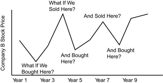
What if we wanted a little more confidence as to potential outcomes? What if we wanted more than 68 percent confidence? What is the likelihood that an observation would fall within a range of plus or minus two times the standard deviation (within two standard deviations)? In the case of Company B, that would mean within a range of a $6.11 million profit and a $6.11 million loss. The likelihood of seeing an outcome fall inside of that range would be 95 percent. Again, the precise derivation of these percentages is a function of standard deviation and isn’t vital to our using them to understand standard deviation and volatility. Given that 95-percent likelihood, it’s not surprising that Company B didn’t have any years outside that range. And if we wanted even more assurance? The likelihood of any observation falling inside of three standard deviations is over 99 percent. Figure 3.2 shows the probability of any outcome falling within these standard deviation ranges.
FIGURE 3.2 Expected Outcome Ranges for Standard Deviation
It’s important to note that these likelihoods, 68 percent, 95 percent, and 99 percent, are valid for any standard deviation but that the standard deviation might change over time, meaning that the range we’d expect 68 percent of all outcomes to fall into would also change. If Company B fired Swing-for-the-Fences Freddy as CEO and replaced him with Steady Eddie, formerly the CEO of Company A, then we would expect the future outcomes for Company B to change. A company’s fortunes rarely change that drastically, however, so it’s generally fair analysis to expect the past to repeat itself to a certain degree.
STANDARD DEVIATION OF RETURNS IS VOLATILITY
In the context of options and their underlying assets, volatility is simply the annualized standard deviation of daily percentage changes in the price of the underlying. Just as with the earnings for Companies A and B, if the price of a stock changes very little over time, then that stock price displays a low standard deviation of percentage daily changes and low volatility. If the price of a stock changes a great deal from day to day, then that stock price displays a high standard deviation of daily price changes and a high volatility.
Since volatility in finance is in annualized terms, the volatility of any stock or underlying is the range of annual price changes we’d expect to see 68 percent of the time. If a stock had a volatility of 20 percent then in about two of every three years (actually 68 percent of all years) we’d expect the stock to have risen less than 20 percent or to have fallen by less than 20 percent. It doesn’t mean it couldn’t move more than 20 percent, it just means that we’d expect that sort of outsized movement only 32 percent of the time.
It’s important to remember that the standard deviation that we use as volatility in option trading is the annualized standard deviation of the daily percentage price changes of the underlying and not the standard deviation of the absolute price or the absolute price change. This is an important difference. Let’s look at two new companies, Company C and Company D, selling at the prices shown in Table 3.1.
Table 3.1 Daily Stock Prices for Company C and Company D
| Day | Company C | Company D |
| IPO Price | 100.00 | 25.00 |
| 1 | 101.00 | 25.25 |
| 2 | 100.50 | 25.50 |
| 3 | 99.75 | 24.75 |
| 4 | 100.25 | 25.25 |
| 5 | 100.00 | 25.00 |
Both of the companies saw their stock prices end up just where they started. But how volatile were the prices? The stock price of Company C changed by as much as $1.00 while the price of Company D changed by a maximum of only $0.75, but this isn’t the best measure of volatility.
The standard deviation of the change in price of Company C stock after the IPO is $0.73. We’d expect that 68 percent of observations of the daily net change would fall inside a range of a $0.73 gain and a $0.73 loss.
The standard deviation of the change in price of Company D stock after the IPO is $0.50. We’d expect that 68 percent of observations of the daily net change would fall inside a range of a $0.50 gain and a $0.50 loss.
Does this mean that Company D is less volatile (i.e., less risky) than Company C? No. In this case the net change isn’t the right measure. Take this to its logical extreme. What if Company C saw the same percentage changes but the stock had issued at $10,000 per share solely because Company C had executed a 1 for 100 stock split prior to the IPO? Nothing has changed except the number of shares outstanding and subsequently the price per share. The company, the prospects, and the employees are all unchanged with an IPO price of $10,000 per share. The daily net change in dollar terms would be huge; if we did that calculation the standard deviation of the daily net change in stock price would be $72.89. Would we really say that Company C became 100 times more risky just because of a stock split? Certainly not, because in this situation real risk isn’t equal to the maximum potential loss any more than it is for our U.S. government bond. The better measure is the standard deviation of percentage changes for each day.
Given the difference in absolute stock prices, the percentage of the price change is obviously more informative; a $1.00 change in a $100 stock is small compared to a $0.75 change in a $25 stock. The volatility that we’ll discuss is the standard deviation of the daily percentage price changes.
The standard deviation of the percentage daily change, then, is the best measure of volatility and risk. For Company C it’s 0.727 percent. For Company D it’s 1.981 percent. That makes more sense; Company D is certainly more volatile and riskier than Company C from a subjective point of view. On any given day the distance in percentage terms that Company D is from its IPO price is likely to be greater than for Company C.
A final note about the standard deviations of companies C and D: They don’t define the volatility of the stocks (as we’ll discuss them in the context of options) only because the volatility in the context of options is the annual volatility. We can calculate an annual volatility from these daily numbers, and the formula for that is in the Appendix. If we did that option math we’d find that the annualized volatility of Company C is 11.74 percent. The annualized volatility of Company D is 31.99 percent.
TYPES OF VOLATILITY
We’ve been using the volatility of historical prices for our hypothetical companies. Thus, we’ve been talking about the historical volatility or the volatility realized by these stock prices during these hypothetical historical periods. We can only determine this historical or realized volatility in hindsight. Only by looking at the actual results and then doing the calculation can we find what the volatility actually was.
The fact that the annualized volatility of Company D over those few days was 31.99 percent doesn’t mean that it will be 31.99 percent for the entire year or even that it will stay at 31.99 percent for the rest of the month. The fact that a company’s volatility was 20 percent last year doesn’t mean that we know what it will be for the coming year any more than a stock being up 10 percent last year tells us anything about what it’s going to do next year. In order to know the actual volatility that’s realized during the coming year we’d have to know what the underlying prices were going to be for that year. That’s obviously not possible. This sort of historical volatility is only knowable in hindsight.
We’ve seen that the real value of an option is driven by the volatility of the stock price. This means that if we use the historical volatility of the stock we would know what an option with a term covering that same time period should have been worth. That doesn’t help us today if we’re trying to figure out what an option will be worth in the future. In order to know what that option will be worth, we have to know what the volatility of the underlying stock will be over that term. We need to forecast what the volatility will be.
Forecast Volatility
It makes sense to look at the past to help us figure out the future. A good place to start might be to look at the historical volatility of the stock or underlying asset and then make some adjustments based on events that have already occurred or that will occur. We might think that a stock will be more volatile than the long-run average because of an upcoming earnings announcement. Maybe there’s a new product launch that’s expected. We might think a stock will be less volatile than the long-run average because it now has solid management after years of turmoil.
The forecast volatility that we seek is the volatility over the period from now, or from when we initiate our option position, until the expiration of that option.
Future Volatility
The future volatility is what the actual distribution of observed prices will be in the future. Just as the historical prices can be used to calculate the historical standard deviation of returns, if we knew future prices we could calculate what the actual future volatility of the underlying stock is. This is certainly impossible. But just as we can use historical volatility to find out precisely what an option would have been worth over that historical time frame, if we have the future volatility then we could precisely determine what an option would be worth over that future period.
In our previous example, we bought an option that we thought was going to expire worthless yet we managed to make it pay off. How does that work? The future volatility of that stock was tremendous. It rallied from $100 to $150 in one day and fell back to $50 the next. This future volatility meant that the call option we bought was worth significantly more than we paid for it. We would have been willing to pay up to $99 dollars for it since it allowed us to short DEF stock at $150 (we probably couldn’t have stomached shorting the stock without owning the call option and our broker probably wouldn’t have let us short it after that rally) and to subsequently buy it back at $50.

- Risk isn’t defined by the amount invested. If it were then $1,000 invested in a Treasury bill would be just as risky as $1,000 invested in the highest of high-flying venture capital investments.
- Risk is volatility and volatility is risk because volatility increases the likelihood of an investment being unprofitable at any particular point in time. This is because volatility takes direction, magnitude, and speed into account.
- Volatility will change over time, sometimes for reasons we expect and sometimes for reasons we don’t expect. As companies grow, die, expand, divest, fail, and merge the volatility of their results and stock prices will ebb and flow.
- Risky assets will be cheaper than nonrisky assets because investors demand extra return for taking additional risk. The extra return is generated from a discounted stock price. The risk also increases the value of options because it increases the value of being able to wait and make a better informed decision.
- Volatility is calculated as the standard deviation of price returns. It measures how diverse outcomes are. Wildly diverse outcomes show a high standard deviation of returns. Standard deviation tells us what range of outcomes to expect.
- Risk and volatility are not necessarily bad. They’re tools, and like any other tool they can help or hurt. The Colt .45 helped to tame the West; some settlers also managed to shoot themselves in the foot with it.