CHAPTER 4
Option Pricing Models and Implied Volatility
There are a nearly infinite number of variables we could analyze in trying to determine what an option is worth. We would look at the exercise price and whether it’s a call or a put. We’d certainly consider the expiration date, but we could also examine the fundamentals of the underlying stock, including its competitive position in its industry. We could examine its balance sheet, including cash on hand and accounts receivable. We could look at the stock’s chart over time to find important technical levels. We could look at the medical history of the CEO to try and divine if he’s likely to drop dead of a heart attack soon. Even if we could figure the odds of such a heart attack, we’d then have to figure out whether such a change in leadership would be a good thing (Swing-for-the-Fences Freddy from Company B) or a bad thing (Steady Eddie from Company A). The result would be so much analysis that we’d experience paralysis.
Instead of looking at everything, we might look at fewer inputs, just enough inputs to help us make some decisions. And since all the fundamental, technical, and even medical information is supposed to help us understand and measure risk, we could use a single proxy for risk. As we discussed in the Chapter 3, that risk measure is volatility.
IT’S AN OPTION PRICING MODEL, NOT AN EQUATION FOR OPTION VALUES
What do we have when we reduce the size and scope of a problem so that solving it becomes manageable? We have a model. Models, whether mathematical ones to help us understand options or plastic ones created by an architect to help us visualize a new building, necessarily eliminate certain considerations in an effort to isolate and emphasize the most meaningful considerations. The result is that a model can help us make certain decisions but can’t make those decisions for us.
The original option pricing model was created by Fischer Black and Myron Scholes and is still the best-known model today. The Black-Scholes model was so vital to the growth of listed option trading and so completely highlights the important inputs in option trading that it’s the only equation we’ll discuss outside of the Appendix.
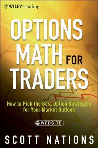
The Black-Scholes price for a call option is:
![]()
Where:
| And where: | S is the price of the underlying stock |
| SK is the strike price of the call option | |
| r is the annual risk-free interest rate | |
| Vol is the volatility or the annualized standard deviation of underlying stock returns | |
| t is the time to expiration (in annual terms such that 6 months is 0.5) | |
| e is the base of the natural log and is equal to 2.7183 | |
| ln is the natural logarithm | |
| N represents the cumulative standard normal distribution. This cumulative distribution describes the probability of a random variable falling within a certain interval. The cumulative distribution value for any number can be found in online tables or can be calculated using a spreadsheet. |
The Black-Scholes equation for the price of a put option is similar but slightly different. That equation can be found in the Appendix.
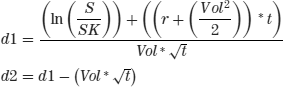
A BLACK-SCHOLES EXAMPLE
Let’s assume:
How much would this call option be worth?
THE ASSUMPTIONS
Since all models are simplified versions of real-world situations, they have to make assumptions about how the world works. For the Black-Scholes model the assumptions about how our little world works include:
- The underlying stock pays no dividends during the term of the option. This obviously makes it tough to use Black-Scholes if the underlying we’re interested in does indeed pay a dividend, but the assumption eliminates the need to account for changes in option prices resulting from payment of a dividend. It also eliminates concerns about the time value of money as it applies to the timing of the dividend.
- The option can only be exercised on the expiration date. As we’ve learned, that means these are European-style options while most options on stocks and ETFs are actually American-style, meaning they can be exercised at any time. The extra freedom associated with early exercise means that American-style options are slightly more valuable than European-style options. The difference is usually pretty small because it’s rarely advantageous to exercise earlier than we have to (early exercise to capture a dividend that’s about to be paid is theoretically the only situation in which early exercise would be advantageous), but eliminating the complexity of the potential for early exercise was necessary for the first option pricing model because the ability to early exercise really means we have an infinite number of very short-term options.
- Underlying markets are efficient. This means that direction can’t be predicted consistently.
- No commissions are charged.
- Risk-free interest rates are known and remain constant over the life of the option, and we’re freely able to borrow and lend at this risk-free rate. While interest rates are known when we price our option it’s likely that they’re going to change over the life of our option. The impact of changes in interest rates on option prices is usually pretty small, but this assumption explains why a simplified model of the option world was necessary. There are an infinite number of paths that interest rates could take over the life of our option. To account for each of those infinite paths would be an incredibly involved undertaking. It’s just easier to eliminate that consideration.
- Volatility is constant. This is the most significant assumption. The thought that the volatility of the underlying asset is fixed for the term of our option is obviously at odds with the real world. Stocks get incredibly volatile just before and just after earnings are announced and when major economic news is released. Stocks tend to be much less volatile in the weeks after earnings come out. However, as there are infinite paths that interest rates can take during the term of our option, there are infinite paths that the volatility of the underlying can take during the life of our option.
- It is always possible to buy or sell any amount of stock, even fractional shares, and stock prices are continuous, meaning there are no jumps or gaps. This is the assumption that many traders believe is most divorced from the real world. Clearly, it’s not possible to trade fractional shares, and stocks clearly experience gaps and jumps. In the real world faced with jumps and gaps, option traders have introduced so-called fudge factors to option pricing. One of the most important fudge factors is skew, discussed in Chapter 6.
- Underlying asset prices are lognormally distributed. A lognormal distribution has a longer right tail, representing prices increasing, and a shorter left tail, representing prices decreasing, than a normal, bell-shaped distribution. The lognormal distribution acknowledges that stock prices will exist between zero, since stock prices can’t be negative, and infinity, and acknowledges as well that stocks have an upward bias, since companies should be creating value over time. Thus, the lognormal distribution also acknowledges that stock prices can drop by 100 percent but can increase by more than 100 percent. In reality, stock price distributions are often not lognormal. They tend to have faster, larger drops than expected.
The fact that these assumptions don’t comport with the real world results in some unusual phenomena that we’ll discuss in Part Two. Savvy option traders can use these phenomena to their advantage.
INPUTS TO THE BLACK-SCHOLES OPTION PRICING MODEL
Almost all of the inputs to the Black-Scholes model are easily knowable: Strike price, put or call, and expiration are absolutely knowable. We know what the risk-free interest rate is (most traders use the 1-month or 3-month Treasury bill rate). The only input that might give us a little pause is volatility. Even with that one we might think that if we just figure out how volatile this stock was in the past, then we’ll know how volatile it will be for the life of our option. This would be the historical volatility we discussed in Chapter 3. However, as we’ve already discussed, the volatility of a stock can change over time: Remember when our hypothetical Company B decided to fire Swing-for-the-Fences Freddy and replace him with Steady Eddie? If we used the historical volatility of Company B then we’d be using a volatility input that was higher than the actual volatility of Company B would be for the life of our option. We’d end up thinking options on Company B were worth more than they ultimately would be. If we relied on historical volatility as our input, we would constantly be a buyer of Company B options and we would constantly be disappointed because they would end up being worth less than we paid.
In our example of Black-Scholes we originally used a volatility input of 20 percent. This was a guess of what the volatility would be for the 60-day term of our option because it was the historical volatility for the underlying stock for the previous 60 days.
The result of using historical volatility is to calculate how much an option would have been worth if its life had matched the timeframe for the historical price data we have. We ended up figuring out what this option would have been worth 60 days ago. Knowing how much such an option would have been worth won’t do us much good in trying to figure out how much our option is worth right now.
Black-Scholes is a model that we can use to help us make sense of the world; in our case it’s the world of options on our underlying. But there’s a reason we call it a model and not an equation even though there’s an equals sign in there. Black-Scholes does not tell us what an option will be worth. It tells us what an option would be worth if the volatility input we chose ended up being precisely equal to the realized volatility for the term of our option, and if all those assumptions held.
IMPLIED VOLATILITY
We can look online and see option prices; someone obviously manages to come up with a price because options trade. Since we can see the option prices and since all the inputs to Black-Scholes, except volatility, are known, can’t we reverse engineer the volatility the market is using? In our example we used a volatility of 20 percent to come up with a call option value of 1.02. We calculated our estimate of the value of the call option as follows:
What if we see that the price of that call option in the market is actually 1.25? We could work backward, relying only on those variables that are either directly certain (e.g., strike price, time to expiration) or observable (e.g., underlying price, risk-free rate, observed value of the option) and do the option math like this:
This way we generate a volatility input implied by the observed option price of 23 percent.
The previous forms of volatility that we’ve discussed—historical and forecast—relate to the underlying and to changes in the underlying prices. Implied volatility relates to the option. It’s the reverse-engineered volatility that is implied by observed option prices.
THE SENSITIVITY OF OPTION PRICES TO CHANGES IN THE INPUTS
What would happen to an option price if we changed one of the inputs? The inputs that could change during the life of our option include the underlying stock price, time to expiration (not only could this change, it has to change), the risk-free interest rate, and implied volatility. They wouldn’t be in the option pricing model if they weren’t important, but do they impact an option’s price? We can use that same Black-Scholes option pricing model to determine how sensitive our option price would be to changes in these inputs.
Together, these sensitivities, along with some others that are incredibly technical, are referred to as the Greeks because we use Greek letters and glyphs as shorthand references to each. Delta, an option’s sensitivity to changes in the price of the underlying, is the most important sensitivity measure for directional traders. Theta refers to an option price’s sensitivity to changes in time to expiration. It’s really an option price’s change (decrease) due to the passage of a single trading day. Gamma is a measure of how quickly delta, an option’s directionality, changes, and Vega is the measure of an option’s sensitivity to changes in implied volatility.
Delta
An option’s value obviously changes as the price of the underlying stock changes, but by how much will it change? That measure is known as delta and it’s easily the most important of the Greeks for the directional, nonprofessional option trader.
If our underlying stock is trading at $1 and we have a 100 strike call option expiring soon, then a small change in the stock price is going to have almost zero impact on the value of our call option. The underlying stock is so far away from our strike price, and is so unlikely to ever get to our strike price given that it expires soon, that even a doubling of the stock price from $1 to $2 would have exceedingly little impact.
On the other hand, if our underlying stock is trading at $1,000 and we have a 100 strike call option, then even a small change in the stock price is going to have an equal change in the price of our call option; our call option has become a proxy for the underlying stock since the likelihood of our option being in-the-money at expiration is huge. If the stock price rose to $1,001 then the value of our option would also increase by $1 (our option would move in price from $900 to $901 since there would be zero time value for such an option).
Delta, the sensitivity of an option price to changes in the price of the underlying, is tiny for a very out-of-the-money option and is huge for a very in-the-money option. What about for the sort of options we generally encounter, an option that’s at-the-money, or nearly so?
One way to think about delta is to consider it the likelihood that an option will expire in the money. In our first example with the stock at $1 and a 100 strike price, that was very unlikely, and so that option had a minuscule delta. In our second example, with the stock at $1000 and a 100 strike price, it was almost certain that our option would expire in-the-money, so that option had a very large delta. What is the likelihood that a 100 strike call will expire in-the-money if the underlying stock is trading at $100? In this situation it’s nearly a coin flip because over a short period we don’t really know in which direction a stock is going to move. The odds of any particular outcome of a coin flip, say heads, is 50 percent. If our option is precisely at-the-money, then the odds of any particular outcome at expiration (in-the-money or out-of-the-money, since precisely at-the-money is a little like expecting a flipped coin to land on its edge), is also 50 percent. The sensitivity of our at-the-money option to any change in the underlying would be 50 percent of that change so the delta for this option would be 50. If our 100 strike call was trading at $5.00 with the underlying stock at $100, and the underlying stock rose by $0.80 to $100.80, we’d expect our call option price to increase by 50 percent of that $0.80. We’d expect our call option to now be worth $5.40.
In our implied volatility example (with volatility at 23 percent) the delta is 40, meaning that if the underlying stock moved from $48.60 to $49.60 we’d expect the price of the call option to change by 0.40, from 1.25 to 1.65.
Theta
Theta is the sensitivity of an option price to changes in time to expiration. It’s the change we’d expect to see in an option price—since we’re only getting closer to expiration it’s the decrease we’d expect to see due to the passage of time. Since options are a wasting asset, theta is where the rubber meets the road. In our example with an implied volatility of 23 percent we’d expect the price of our call option to decrease in value by 0.015 today. Observant readers will note that 0.015 multiplied by 60 days doesn’t get us our observed option price of 1.25. Theta increases as expiration nears, and we’ll discuss that more in Chapter 7 because we can use that increase to our advantage.
Gamma
When discussing delta we saw that the delta for our deep out-of-the-money option was zero. The delta of the at-the-money option was 50. The delta of the deep in-the-money option was 100. Delta obviously changes as the underlying price changes. Gamma describes this rate of change. For the professional trader who’s stripping the directionality from their option position by taking an offsetting position in the underlying and using the delta to determine what the size of that offsetting position should be, gamma is their risk or reward.
In our example with an implied volatility of 23 percent, the gamma of our call option is 0.085. This means that for each 1-point change in stock price we’d expect the delta of our option to change by 0.085. If the stock rallied we’d expect the delta to increase, and if the price of our stock fell we’d expect delta to decrease. If our stock rallied by 1 point to $49.60 we’d expect the delta to be 48.5(40 plus 8.5). That makes sense because with the stock price just below the strike price of our option, and with 60 days left to expiration, the odds of our call option expiring in-the-money are nearly 50/50.
Vega
Volatility is the most important input to any option pricing model and, as we’ve said, it’s impossible to know what the correct input is until after the option has expired. If the market’s estimation of what volatility will be changes, then traders will manifest this by changing option prices. The impact of the change in implied volatility on an option’s price is vega. Vega assumes implied volatility changes by 1 percent (say from 23 percent to 24 percent in our example) and reflects the sensitivity of the option price to that 1 percent change in implied volatility.
In our example with implied volatility at 23 percent, the vega was 0.076, meaning that a change in implied volatility from 23 percent to 24 percent would increase the price of our call option by $0.076, from $1.25 to $1.33.
Rho
Delta, theta, gamma and vega are the most important Greeks but an option’s price is sensitive to other changes as well. One example is interest rates. Despite the assumption inherent in the Black-Scholes model, interest rates are likely to change during the term of options. Rho is a measure of the impact of the change in interest rates, specifically the interest rate we’ve used in our pricing model, on the price of an option. It’s not possible to generalize on the impact of changes in interest rates on option prices. Rho depends on issues like the type of option (American-style or European-style) and the type of underlying asset, as well as others. The formulas for all these sensitivities can be found in the Appendix.
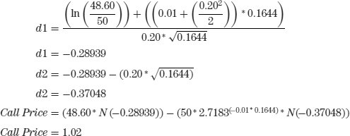
These sensitivities can be overwhelmed by each other. The passage of time (theta) might take more out of an option’s value than a mildly increasing implied volatility (vega) can add. Likewise, a call option may become less valuable despite a rising underlying if implied volatility is falling enough or due to the passage of time. Similarly, implied volatility can increase so much that an option is worth more than it was the previous day despite time decay. In this situation, time didn’t run backward, the erosion occurred but it was overwhelmed by the increase in implied volatility. Figure 4.1 shows the general response to option prices due to changes in the price of the underlying, changes in implied volatility, and as well to the passage of time.
FIGURE 4.1 Option Sensitivities
These sensitivities are rules of thumb, not immutable laws of nature, but they can be used over time to inform our trading decisions. We’ll learn how to do that in Part Three.

- Lots of variables can be used in determining an option’s value. We’ll focus on a few quantifiable variables.
- An option pricing model, even though it’s a mathematical calculation, is not a magic equation that tells you how much an option is worth now or how much it’s going to be worth at expiration. Use the tools at OptionMath.com but remember that these tools should be used as a map, not an autopilot.
- Option pricing models make many assumptions: Some relate to dividends, others to how the underlying market functions, how interest rates will change, what volatility will be, what sort of distribution of returns the underlying will display, and so forth.
- None of these assumptions are valid in the real world. All are contrary to the way the world really works.
- We can still use assumptions. In fact, the way the market responds to these assumptions can be used to our advantage. We’ll learn how to do that in Part Three.
- Implied volatility is the volatility of the underlying asset, for the term of the option, implied by the observed option price. Think of using the Black-Scholes model, inserting the observed option price and solving backward for the volatility input.
- Changes in the underlying price, time to expiration, and implied volatility will change option prices. The Greeks quantify these sensitivities.