CHAPTER 14

Vertical Spreads

Just as a risk reversal takes advantage of skew to get bullish exposure to the underlying stock, vertical spreads can take advantage of skew, and some of the other phenomena we’ve discussed, to get bearish exposure to the underlying.

A vertical spread is executed when you buy one option and sell another option of the same type (put or call) and the same expiration date but with a different strike price.

While vertical spreads, sometimes simply called verticals, can be either bearish or bullish, skew is generally working against a bullish vertical spread, whether it’s a call spread or a put spread, so we’ll focus on bearish vertical spreads.

Since we’re focusing on bearish vertical spreads in order to take advantage of skew we’ll look at buying a put spread (buying the strike price that is closer to at-the-money and selling the strike price that is further from at-the-money) and at selling a call spread (selling the strike price that is closer to at-the-money and buying the strike price that is further from at-the-money). Table 14.1 shows two bearish vertical spread examples for IBM stock.

Table 14.1 Bearish Put and Call Vertical Spread Examples

IBM	206.81
Put Spread	Option Price
Buy July 200 Put Option	4.30
Sell July 180 Put Option	1.00
Net Premium Paid	3.30
Call Spread
Sell July 210 Call Option	4.80
Buy July 230 Call Option	0.50
Net Premium Received	4.30

In buying the July 180/200 put spread our trader would buy the July 200 put at $4.30 and sell the July 180 put at $1.00. The total paid for the spread is $3.30.

In selling the July 210/230 call spread our trader would sell the July 210 call at $4.80 and buy the July 230 call at $0.50. The total received for selling the spread is $4.30. The benefit of selling a call spread is that the upper strike call, in this case the 230 call, caps the risk from what would otherwise be a naked call in selling the 210 call.

The minimum value of any vertical spread is zero; no vertical spread can have a negative value because no one would be willing to pay more for a lower strike put or more for a higher strike call. The minimum value of both of these IBM vertical spreads is zero.

The maximum value of any vertical spread is the distance between the strike prices. The maximum value of this IBM put spread is $20.00 because 200 minus 180 equals 20.00. The maximum value of this IBM call spread is $20.00 because 230 minus 210 equals 20.00.

BREAKEVENS

The breakeven point for a short call spread is very similar to the breakeven for a short call. The underlying stock can rally, at expiration, to a price equal to the strike price of the short call leg of the spread plus the amount of total premium received. At this point, the spread our trader is short is worth precisely the premium received.

The breakeven for a long put spread is likewise similar to the breakeven for a long put. At expiration the stock has to have fallen below the strike price of the long option portion of the spread by enough to pay for the spread. The breakeven point is that long strike price minus the total amount of premium paid. At this point, the spread our trader is long is worth precisely the price paid for it. (See Table 14.2.)

Table 14.2 Put and Call Vertical Spread Breakeven Points

Put Spread
Buy July 180/200 Put Spread	3.30
Breakeven Point	196.70
Call Spread
Sell July 210/230 Call Spread	4.30
Breakeven Point	214.30

SKEW AND VERTICAL SPREADS

Because skew can have such an impact on option prices and since there’s no reason to be swimming against the current, when using vertical spreads we’ll focus on buying put spreads or selling call spreads. Table 14.3 shows what our IBM vertical spreads would be worth if it weren’t for skew.

Table 14.3 Put and Call Vertical Spread Examples Without Skew

	Observed Price	What That Price Would Have Been without Skew
Put Spread
Buy July 200 Put Option	4.30	4.05
Sell July 180 Put Option	1.00	0.32
Net Premium Paid	3.30	3.73
Net Benefit from Skew		0.43
Call Spread
Sell July 210 Call Option	4.80	4.94
Buy July 230 Call Option	0.50	0.72
Net Premium Received	4.30	4.22
Net Benefit from Skew		0.08

In both the put spread bought and the call spread sold, skew generated a net benefit. There would certainly be other phenomena that would be helping or hurting these trades. The volatility risk premium would be helping the call spread since our trader would likely be selling the 210 strike call for more than it was worth, and that benefit would probably overwhelm the damage that the volatility risk premium would do to the profitability of the 230 strike call option bought. Time decay would also likely help the profitability of the call spread, since the daily erosion received from the call our trader is short (the 210 strike call) is going to be greater than the daily erosion paid on the option our trader is long (the 230 strike call).

The volatility risk premium is likely to hurt the profitability of the put spread bought, since the volatility risk premium paid in the 200 put is likely greater, in dollar terms, than the volatility risk premium received in the 180 put. Of course, it’s not possible to know what the volatility risk premium will ultimately be for any of these options. That would require knowing what the realized volatility of IBM stock will be for the term of these options.

Time decay will also likely hurt the profitability of the put spread bought, since the daily erosion paid in the 200 put is going to be greater than the daily erosion received in the 180 put. Table 14.4 shows the daily erosion (theta) for each of these options and spreads.

Table 14.4 Daily Erosion of Vertical Spreads

	Daily Erosion
Put Spread
Buy July 200 Put Option	0.039 Paid
Sell July 180 Put Option	0.021 Received
Net Daily Erosion	0.018 Paid
Call Spread
Sell July 210 Call Option	0.038 Received
Buy July 230 Call Option	0.013 Paid
Net Daily Erosion	0.025 Received

A Word About Terminology

Many books refer to bull call spreads and bear put spreads and vice versa but option professionals rarely use these terms. Rather they buy or sell the spread and the spread is a put spread or a call spread. This is the terminology we’ll use and that you can see in Table 14.5.

Table 14.5 Vertical Spread Terminology

Action	Market Outlook	Structure
Buy a Call Spread	Bullish	Buy Closer to At-the-Money Call, Sell More Out-of-the-Money Call
Sell a Call Spread	Bearish to Neutral	Sell Closer to At-the-Money Call, Buy More Out-of-the-Money Call
Buy a Put Spread	Bearish	Buy Closer to At-the-Money Put, Sell More Out-of-the-Money Put
Sell a Put Spread	Bullish to Neutral	Sell Closer to At-the-Money Put, Buy More Out-of-the-Money Put

The benefit of using this terminology is that it’s aligned with that of buying or selling outright puts and calls.

VERTICAL SPREAD RISK AND REWARD

One reason the smart trader will use vertical spreads is that they define the potential risk of the trade. The maximum risk for any long vertical spread is the total paid for it. In our first IBM example, buying the July 180/200 put spread for $3.30, the maximum potential loss is the $3.30 paid.

The maximum potential loss for any short vertical spread is the distance between the strike prices, often referred to as the width of the spread, less the premium received. In the IBM call spread example, the maximum potential risk is $15.70, which is the $20.00 width of the spread minus the $4.30 in premium received.

In addition to getting some of the phenomena working to our advantage and mitigating the damage from those that are working against us, buying a vertical spread can significantly reduce the cost of a trade. For example, the IBM put spread only cost $3.30 or nearly 25 percent less than simply buying the July 200 put outright would have cost. The downside of this lower cost is that the potential profit is limited, just as the potential risk is limited. For a long vertical spread the maximum potential profit is the width of the spread minus the amount paid for the spread. (See Table 14.6.)

Table 14.6 Risk and Reward for Vertical Spreads

	Maximum Risk	Maximum Reward
Short Vertical Spread	Width of the Spread Minus the Net Premium Received	Net Premium Received
Long Vertical Spread	Net Premium Paid	Width of the Spread Minus the Net Premium Paid

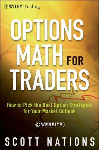
In the IBM put spread example the maximum potential profit would be $16.70, which is the $20.00 width of the spread minus the $3.30 paid. For a short vertical spread the maximum potential profit is the net premium received for selling the spread. In this way a short spread is identical to a short outright option position, the maximum potential profit is the premium received.

What would the risk and reward of buying this IBM put spread look like? Figure 14.1 shows the payoff chart for buying the IBM put spread.

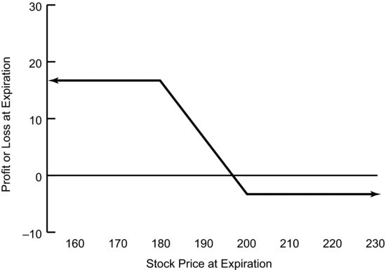
In the IBM call spread example, our trader sold the 210 call at $4.80 and bought the 230 call at $0.50. The net premium received was $4.30. That $4.30 would be the maximum potential profit. The maximum potential loss would be $20.00 (the width of the spread) minus $4.30 (the net premium received) or $15.70. Figure 14.2 shows the payoff chart for selling the IBM call spread.

LONG PUT SPREADS AND SHORT CALLS SPREADS ARE ALIKE

Long put spreads and short call spreads are alike in many ways, but that doesn’t mean they’re identical. We’ve already seen how the risk and reward for each is different but they are alike in important ways such as market outlook and in ways that are a result of the phenomena we discussed in Part Two.

Both Are Bearish

Long put spreads and short call spreads are similar in that both are bearish. They both want the price of the underlying stock to drop, although a short call spread can also realize its maximum profit if the stock does not move, but both spreads lose money if the underlying rallies sufficiently. If the market rallies the long put spread will lose the amount of premium spent and the short call spread will lose the width of the spread minus the premium received.

Both Use Skew

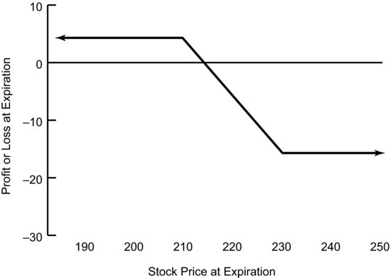
Bearish verticals are also similar in that both can use skew. Nearly any long put spread will find that skew is advantageous because it’s almost always the case that a put strike that is closer to at-the-money is going to have a lower implied volatility than a put strike that is more out-of-the-money. Figure 14.3 shows the skew curve for these IBM July options.

The put spread is buying the 200 strike put at an implied volatility of 17.79 percent and selling the 180 strike put at an implied volatility of 22.34 percent. The call spread is selling the 210 strike call at an implied volatility of 16.28 percent and buying the 230 strike call at an implied volatility of 15.48 percent. Again, Table 14.3 quantified this impact in dollar terms.

Both Are Always Bearish

As we saw in calendar spreads, some directional positions can change their directionality. Bullish calendar spreads that originally need the underlying to rally can see the underlying go too far and find that their maximum profit is achieved if the underlying falls back. This isn’t the case with bearish vertical spreads. They’re both always bearish although, at some point, a bearish move in the underlying ceases to generate additional profit. This occurs if the spread is already at its point of maximum profit. For a long put spread it occurs if the underlying is below the bottom put strike price by an amount sufficient to wring all the time value out of both options. The same is true for a short call spread. Once this point has been reached by the underlying, any continued drop in price does no good. The put spread can’t be worth more than the width between the strikes, and the call spread can’t be worth less than zero.

LONG PUT SPREADS AND SHORT CALL SPREADS ARE DIFFERENT

A much as long put spreads and short call spreads are alike, they’re also different in important ways. First, a short call spread is risking a lot to make relatively little but should expect to be profitable fairly frequently. On the other hand, a long put spread is risking a little to make a lot and, as such, we should expect it to be profitable much less often. We should expect it to realize its maximum profit potential even less often.

How often will a short call spread end up fully in-the-money with the underlying above the upper strike price at expiration? This question is important because it’s at this point that the call spread realizes its maximum potential loss. That likelihood would be the delta of that upper call option. For the short IBM call spread that delta is 9, so the likelihood of sustaining the maximum potential loss is 9 percent.

How often will a long put spread end up fully out-of-the-money so that the underlying is above the top put strike at expiration? The delta of the top put strike is the likelihood it’s in-the-money at expiration. We’d sustain the maximum loss if it’s out-of-the-money at expiration. What would that number be? It’s simply 1 minus the delta. The delta of that 200 put is 33. Thus, the likelihood of the put spread sustaining its maximum loss, with IBM above $200 at expiration, is 67 percent.

Table 14.7 shows the risk, the reward, and the likelihood of each.

Table 14.7 The Likelihood of Sustaining the Maximum Loss

These likelihoods of realizing the maximum loss aren’t the likelihood of sustaining any loss. While the likelihood of the short call spread sustaining the maximum loss is only 9 percent, that would require IBM to be at or above $230 at expiration. Since the breakeven for this trade is $214.30, what’s the likelihood of IBM being above $214.30 at expiration? That’s the likelihood of this trade sustaining any loss if our trader holds it to expiration. Obviously there’s no option with a strike price precisely equal to $214.30 but we can put that strike price into the option pricing model at OptionMath.com and find out that the delta of a hypothetical $214.30 strike call option is about 37. That means the odds of this trade sustaining any loss is about 37 percent if we hold it to expiration. We’d certainly expect the odds to be in our favor since we’re risking a relatively large loss ($15.70) in order to make a relatively small gain ($4.30).

The long put spread is a little different because we’re risking relatively little ($3.30) to make a relatively large profit ($16.70). Given the difference between the risk and the potential payoff we’d expect to sustain a loss much more frequently than we would with the short call spread. The breakeven for the long put spread is $196.70, meaning IBM has to be at or below $196.70 at July expiration. Again, this probability is the delta of this $196.70 put option. The trade will sustain a loss if IBM is above $196.70 at expiration. The delta of the $196.70 put is 29, so the probability of IBM being above that price at expiration is 71 percent.

THE WIDTH OF THE SPREAD VERSUS THE COST

It’s relatively easy to know whether an individual option is expensive or cheap: We simply look at the implied volatility. Things are a little more difficult for a vertical spread. If we look at the implied volatility of the option that’s closer to at-the-money, then we’d only know whether options in general are expensive or cheap. We wouldn’t know much about a spread because we don’t know how wide the spread is, and we don’t know what impact skew will have on the cost of the spread.

A better way of looking at the cost of a spread is to take into account the cost of the spread versus the width of the spread. The IBM put spread example cost $3.30 and the spread was $20.00 wide. That means the spread cost 16.50 percent of the width of the spread. The IBM call spread example cost $4.30 and again the spread was $20.00 wide, so the spread cost 21.5 percent of the width of the spread.

These ratios are pretty inexpensive given that one strike is so close to at-the-money. That is partly a function of implied volatility in IBM being pretty low. How close one strike price is to at-the-money is also a consideration. Obviously if we selected a spread that was significantly out-of- the-money we’d expect it to be pretty cheap. That means the relationship between cost and width would look significantly different for way out-of-the-money spreads than it does for at-the-money spreads as we see in Table 14.8.

Table 14.8 Moneyness and Cost versus Width

This relationship makes sense, the spread costs less and less as a percentage of the width as it gets further from at-the-money and it’s also less and less likely to be in-the-money at expiration as it gets further from at-the-money. Let’s look at the same probabilities for loss we looked at before. If we bought the IBM July 130/150 put spread at $0.13 with IBM at $206.81 we wouldn’t expect to pay very much, the breakeven is a long way from the current stock price; it’s $149.87, or 27.5 percent below the current price for IBM. We’re risking very little, $0.13, in order to make a great deal, $19.87, so the odds of doing so should be small. Since the delta of the $149.87 strike put would be 2, the probability of losing money is 98 percent. That doesn’t necessarily mean this is a bad trade, it just means a trader buying this put spread needs to have reasonable expectations.

Similarly, selling the 260/280 call spread only generates $0.04 in premium and has a potential loss of $19.96. This is not a trade a sensible trader would make, despite the probability of losing money being very small, given the disparity between the risk and reward. The breakeven for selling this call spread is $260.04, the short strike price plus the net premium received. The delta of a theoretical 260.04 strike call option is very small, about 0.20, so the odds of sustaining a loss are 0.20 percent.

By the way, if we calculate the necessary potential profit to make the trade worthwhile we’d divide the potential profit, $0.04, by the odds of sustaining a loss, 0.20 percent. It’s no accident that the result of 0.04/0.20 percent is 20, the width of the spread. This simply means there’s no purely mathematical advantage to making or not making the trade. Rather, while no trader should make this trade, in a similar situation with a more appropriate payoff but the same lack of mathematical edge, traders will trade if they feel they have an information edge on the direction and magnitude of the trade.

THE GREEKS

Vega—The Effect of Changes in Implied Volatility

Several of the previous strategies we’ve examined are very dependent on changes in implied volatility during the term of the trade. For example, in a covered call or short put, a decrease in implied volatility can generate additional profit before expiration. In a calendar spread an increase in implied volatility will make the remaining option more valuable at the expiration of the short option.

Vertical spreads are generally much less susceptible to changes in implied volatility since any impact on one option is going to have a similar impact on the other leg of the spread. While both options will be impacted to different degrees, the impact will be similar and offsetting. If the spread is very narrow then the effect will be very small but as the spread gets wider the effect will increase.

For example, any change in implied volatility will have a relatively small impact on the IBM put spread we’ve been examining, as seen in Table 14.9.

Table 14.9 Implied Volatility and the Impact on Vertical Spreads

	Option Price	Vega (Change in Option Price Due to 1 Point Change in Implied Volatility)
July 200 Put Option	4.30	0.372
July 180 Put Option	1.00	0.158
Net Vega		0.214
July 210 Call Option	4.80	0.381
July 230 Call Option	0.50	0.140
Net Vega		0.241

A 1-point change in implied volatility will cause a change of $0.372 in the price of the July 200 put option. If implied volatility increased by 1.00 we’d expect the option price to increase to $4.67. If implied volatility decreased by 1.00 we’d expect the option price to decrease to $3.93. Similarly, the July 180 put would change in price by $0.158 for each one-point change in implied volatility. This means that the spread would only change in price by $0.214 for each 1-point change in implied volatility. The change in price of the spread is just more than half what it would be for the 200 put alone. Changes in implied volatility during the term of the spread will certainly change the value of the spread, but not in the major way that the value of a covered call or short put might change.

A 1-point change in implied volatility will cause a $0.381 change in the price of the 210 call option. It will also cause a change of $0.140 in the price of the 230 call option. The net effect on the call vertical spread of a 1-point change in implied volatility would be $0.241.

Delta

Just as the vega of one leg of any vertical spread will offset some of the vega exposure of the other leg, some of the directionality of one leg of a vertical spread will offset the directionality of the other leg. (See Table 14.10.) This directionality is the delta we discussed earlier. The result is that the delta, the sensitivity of an option’s price to changes in the price of the underlying stock, for a vertical spread tends to be pretty small. In the IBM examples it is smaller than the delta of the outright, at-the-money, option.

Notice that the net delta for both spreads is negative, meaning that they’re both bearish. This is what we were trying to accomplish as contrary trades to the bullish risk reversal. This net delta is the change we’d expect to see in the value of the spread if IBM changed in price by $1.00. We’d expect the put spread to change in value by $0.24 and the call spread to change by $0.36; if IBM rallied by $1 we’d expect to see the value of each spread change by that net delta (the put spread would fall, the call spread would rise). If IBM fell by $1 we’d expect to see the value of each spread change by that net delta (the put spread would rise, the call spread would fall). These deltas are only valid over short price ranges and only for today. The deltas will change as the underlying price changes just as they will change as expiration nears.

As vertical spreads get wider each option is a less effective hedge for the other option as we saw in Part Two. Each option will behave differently and the effect of changes in implied volatility and changes in the underlying stock price will be significantly different for each option. As a vertical spread gets wider, the option that is closer to at-the-money starts to act more like an outright option rather than as part of a spread. As the spread gets wider it takes on more directional characteristics becoming more bearish. (See Table 14.11.) We saw this earlier when discussing the angle of the spread and how it affected the ability of one option to hedge another.

The 180/200 put spread is slightly bearish. It makes money if IBM drops and IBM only has to drop 13 percent for this spread to realize its maximum profit. The 150/200 put spread is more bearish. It has a higher maximum profit but IBM has to drop 27 percent for this spread to realize that maximum profit. The 120/200 spread is very bearish. Its maximum profit is much higher but it needs IBM to drop much further, 42 percent, to realize this profit.

Selling the 210/230 call is somewhat bearish; it makes money if IBM doesn’t move or drops but it also has a higher delta than any of the put spreads. The other two call spreads aren’t really spreads at all. Those spreads are much more like selling the 210 call outright since the delta of the spreads is almost identical to that of the outright 210 call.

IMPLIED VOLATILITY AND THE COST OF VERTICAL SPREADS

We’ve already seen that IBM vertical spreads are relatively inexpensive because implied volatility in IBM options, in general, is relatively low. How does the general level of implied volatility change the price of vertical spreads? Table 14.12 shows several hypothetical options and spreads for varying levels of implied volatility. We’ve assumed no skew to remove one variable.

Table 14.10 Delta’s Effect on Vertical Spreads

	Delta
Put Spread
Long July 200 Put Option	−33
Short July 180 Put Option	9
Net Delta	−24
Call Spread
Short July 210 Call Option	−45
Long July 230 Call Option	9
Net Delta	−36

Table 14.11 Bearishness Versus the Width of the Vertical Spread

Table 14.12 Implied Volatility and the Cost of Vertical Spreads

After a certain point, as implied volatility increases the likelihood that both options will expire in-the-money increases, meaning the delta for the spread decreases. The result is that with very high implied volatilities the value of the spread will not change very much given a change in the underlying asset price.

Likewise, after a certain point, as implied volatility increases the net effect of a change in implied volatility (vega) decreases. The result is that, in general, if implied volatility is high a trader is better off either selling outright options such as covered calls or puts to buy stock, or buying vertical spreads such as put spreads. This is also one of the times when buying a call spread, while not generally a way to get the advantage of the option math working in your favor, makes sense.

If our trader doesn’t want to sell outright options in a high implied volatility environment, then he can sell a vertical spread with a short strike price that is very close to at-the-money. Selling a vertical spread with a short strike price that is further from at-the-money blunts the advantage of high implied volatility.

Similarly, if our trader is operating in a low implied volatility environment, it is generally advisable to buy outright options or sell vertical spreads. If our trader wants to buy vertical spreads in a low implied volatility environment, it’s generally a superior strategy to buy a strike price that is closer to at-the-money. Buying a strike price that is further from at the money simply defeats the value of buying a vertical spread in a low implied volatility environment.

VERTICAL SPREADS—HOW AGGRESSIVE?

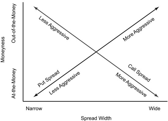
Like nearly all option strategies vertical spreads can be aggressive, moderate, mild, or downright bond-like. The strikes chosen result in spreads that are at-the-money or further out-of-the-money and spreads that are wide or narrow. Since we’re focusing on buying put spreads and selling call spreads, the choices are naturally different. For a long put spread, the spread gets more aggressive as the long strike price gets further from at-the-money because the market has to drop substantially for the spread to go in-the-money, and the trade gets more aggressive as the spread gets wider because the market has to drop substantially before the put spread ceases to participate. For a short call spread the trade gets more aggressive as the short strike price gets closer to at-the-money because the likelihood of the spread going in-the-money increases as the delta of the short strike increases and gets more aggressive as the spread gets wider because the market has to rally substantially before the losses are capped, as Figure 14.4 illustrates.

CALL SPREADS, SKEW, AND THE PROBLEM OF THE “TROUGH”

Skew tends to generate a much smaller benefit for short call spreads than for long put spreads; the difference in implied volatility is lower for call spreads. Our original IBM examples demonstrate this. The benefit from skew for the put spread was 0.43 versus only 0.08 for the call skew. There’s simply less difference in implied volatility for call strike prices than there is for put strike prices. There’s also the possibility in selling a call spread to go out-of-the-money and sell the strike price that is in the bottom of the skew trough we saw in Figure 14.3. For the IBM options that strike price would be the 225 calls with an implied volatility of 15.42 percent. If the call spread we sell uses the 225 strike call as the short leg then skew will actually be working against the spread, as Table 14.13 shows.

Table 14.13 Call Vertical Spreads, Skew, and the Bottom of the “Trough”

The result of selling the strike price that is in the “trough” of the skew curve is that every possible call spread using that strike as the short strike is worse off because of skew.

In selling call spreads it’s generally wise to stick to selling a strike price that is very close to at-the-money. If implied volatility in general is low, low enough that our trader would rather not sell an at-the-money call strike price, then it’s generally wise to look for another strategy altogether, or to recognize the inherent problem and sell a call spread simply because of the payoff profile and the defined risk versus the unlimited risk of selling a naked call option.

Selling the at-the-money call option as part of a short call vertical doesn’t have everything stacked against it. As we’ve discussed, it will usually have the volatility risk premium working for it to some degree. Since the short call option will have greater daily price erosion, the net effect of erosion will also be a positive for a short call vertical.

FOLLOW-UP ACTION

Follow-up action for a vertical spread has, in many ways, already been taken care of. The nature of a spread, particularly a fairly narrow one, limits the potential damage and reduces the need to roll. If the spread is fairly wide then as expiration approaches, and as the strike prices’ ability to hedge each other deteriorates, the need to close the trade or roll one of the strikes might increase. This is only the case if either strike is close to at-the-money, or if one strike is in-the-money and the other strike is out-of-the-money. In this situation the goal of follow-up action is to avoid having an unwanted position in the underlying stock due to exercise or assignment.

If both options will be in-the-money, or if both options will be out-of-the-money at expiration, then little follow-up action is needed. If the options are in-the-money, traders will exercise the option they are long and be assigned on the option they are short. Both spreads will close at their maximum value, the width of the spread. The short call spread will have sustained its maximum loss, but the trade will not generate any position in the underlying stock. The long put spread will recognize its maximum profit and again, there will be no resulting position in the underlying after expiration.

Follow-up action should focus on those instances when one leg of the spread is in-the-money and subject to exercise or assignment and the other leg is out-of-the-money and set to expire worthless. In this situation the spread is going to result in a position in the underlying asset. Given that our trader initiated a spread position, it’s unlikely ending up with a stock position was the goal.

In this situation it’s generally best to close out the trade. In the case of a long put spread that would mean the long put was in-the-money and would result in a short position in the underlying stock, while the short put would expire worthless. Since simply selling the long put would leave our trader naked short a put in an environment where the underlying stock has recently fallen, our trader should sell out the entire spread.

If the short leg of a short call spread is going to expire in-the-money and the long leg is going to expire worthless, our trader would end up with a short position in the stock. In this situation our trader might simply buy back the short call, leaving the worthless long out-of-the-money call to expire, rather than spend the commission to sell it. Since we’re never in favor of selling really cheap options (i.e., worth less than $0.10) we wouldn’t be in favor of selling this worthless, or nearly so, call option. In case of an unexpected development it’s probably a good idea to offer this call for sale at a higher price via a good-till-canceled order as we discussed previously.