Hyperelliptic Curves

Search in book...
Toggle Font Controls
Create new playlist

Name your new playlist

Playlist description (optional)
Sign In

Email address

Password

Forgot Password?

or

Continue with Facebook

Continue with Google
Sign Up

Full Name

Email address

Confirm Email Address

Password

or

Continue with Facebook

Continue with Google

**2.12. Hyperelliptic Curves

Hyperelliptic curves are generalizations of elliptic curves. We cannot define a group structure on a general hyperelliptic curve in the way as we did for elliptic curves. We instead work in the Jacobian of a hyperelliptic curve. For an elliptic curve E over an algebraically closed field K, the Jacobian is canonically isomorphic to the group E(K). Thus one can as well use the techniques for hyperelliptic curves for describing and working in elliptic curve groups. However, the exposition of the previous section turns out to be more intuitive and computationally oriented.

2.12.1. The Defining Equations

A hyperelliptic curve C of genus over a field K is defined by a polynomial equation of the form

Equation 2.13

In order that C qualifies as a hyperelliptic curve, we additionally require that C (as a projective curve) be smooth over . The set of K-rational points on C is denoted as usual by C(K). For g = 1, Equation (2.13) is the same as the Weierstrass Equation (2.6) on p 98, that is, elliptic curves are hyperelliptic curves of genus one. A hyperelliptic curve of genus 2 over is shown in Figure 2.2.

Figure 2.2. A hyperelliptic curve of genus 2 over : Y² = X(X² – 1)(X² – 2)

A hyperelliptic curve has only one point at infinity (Exercise 2.97(f)) and is smooth at . If char K ≠ 2, substituting simplifies Equation (2.13) as . Since is a monic polynomial in K[X] of degree 2g + 1, we may assume that if char K ≠ 2, the equation for C is of the form:

Equation 2.14

Proposition 2.37.

If char K ≠ 2, then the hyperelliptic curve C defined by Equation (2.14) is smooth if and only if v has no multiple roots (in ). If char K = 2, then the curve defined by Equation (2.14) is never smooth.

Proof

First, consider char K ≠ 2. If v has a multiple root, say , then v′(α) = 0 and, therefore, C is not smooth at the finite point . Conversely, if (h, k) is a singular point on , then we have 2k = 0 and v′(h) = 0. Since (h, k) = (h, 0) is a point on C, we have v(h) = 0, that is, h is a multiple root of v.

For char K = 2 and , we have (∂(Y² – v(X))/∂X)(h, k) = v′(h) and (∂(Y² – v(X))/∂Y)(h, k) = 0. Now, v′(X) is a monic polynomial of degree 2g > 0 and, therefore, has at least one root, say . But then C is not smooth at .

Definition 2.82.

Let P = (h, k) be a finite point on the hyperelliptic curve C defined by Equation (2.13). The point is called the opposite of P.^[14] P and are the only points on C with X-coordinate equal to h. If , then P is called a special point on C, otherwise it is called an ordinary point on C. The set of all finite (resp. ordinary, resp. special) points on C is denoted by C_fin(K) (resp. C_ord(K), resp. C_spl(K)). These notations are also abbreviated as C_fin, C_ord and C_spl, if the field K is understood from the context.

^[14] It is customary to define the opposite of to be itself.

2.12.2. Polynomial and Rational Functions

All the general theory we described in Section 2.10 continues to be valid for hyperelliptic curves. However, since we are now given an explicit equation describing the curves, we can give more explicit expressions for polynomial and rational functions on hyperelliptic curves. For simplicity, we consider the affine equation and extend our definitions separately for the point at infinity.

Consider the hyperelliptic curve C defined by Equation (2.13). By Exercise 2.98, the defining polynomial f(X, Y) := Y² + u(X)Y – v(X) (or its homogenization) is irreducible over , so that the affine (or projective) coordinate ring of C is an integral domain and the corresponding function field is simply the field of fractions of the coordinate ring.

Let . Since y² + u(x)y – v(x) = 0 in K[C], we can repeatedly substitute y² by –u(x)y + v(x) in G(x, y) until the y-degree of G(x, y) becomes less than 2. This proves part of the following:

Proposition 2.38.

Every polynomial function can be written uniquely as G(x, y) = a(x) + yb(x) for some a(X), .

Proof

In order to establish the uniqueness, note that if G(x, y) = a₁(x) + yb₁(x) = a₂(x) + yb₂(x), then . Since the Y -degree of f is 2, this implies [a₁(X) + Y b₁(X)] – [a₂(X) + Y b₂(X)] = 0, that is, [a₁(X) – a₂(X)] + [b₁(X) – b₂(X)]Y = 0, that is, a₁(X) = a₂(X) and b₁(X) = b₂(X).

Definition 2.83.

Let . The conjugate of G is defined to be the polynomial function . The norm of G is defined as .

Some useful properties of the norm function are listed in the following lemma, the proof of which is left to the reader as an easy exercise.

Lemma 2.9.

For G, , we have:

.
If G(x, y) = a(x) + yb(x), then N(G) = a(x)² – a(x)b(x)u(x) – v(x)b(x)². In particular, .
.
N(GH) = N(G) N(H).

We also have an easy description of the rational functions on C.

Proposition 2.39.

Every rational function can be written in the form s(x) + yt(x) for some s(X), .

Proof

We can write r(x, y) = G(x, y)/H(x, y) for G, , H ≠ 0. Multiplying both the numerator and the denominator by and using Lemma 2.9(2) and Proposition 2.38 completes the proof.

The value of a rational function on C at a finite point on C can be defined as in the case of general curves (See Definition 2.68). In order to define the value of a rational function at the point , we need some other concepts.

For a moment, let us assume that . From the equation of C, we see that k² ≈ h^2g+1 (neglecting lower-degree terms) for sufficiently large coordinates h, k of a point . This means that k tends to infinity exponentially (2g + 1)/2 times as fast as h does. So it is customary to give Y a weight (2g + 1)/2 times a weight we give to X. The smallest integral weights of X and Y to satisfy this are 2 and 2g + 1 respectively. This motivates us to provide Definition 2.84 (generalized for any K).

Definition 2.84.

Let . The degree of G is defined to be deg G := max(2 deg_x a, 2g + 1 + 2 deg_x b), where deg_x denotes the usual x-degree of a polynomial in K[x]. Since a and b are uniquely determined by G, deg G is well-defined. If G = 0, we set deg G := –∞.

If 0 ≠ G = a(x)+yb(x), d₁ = deg_x a and d₂ = deg_x b, then the leading coefficient of G is taken to be the coefficient of x^d₁ in a(x) if deg G = 2d₁, or to be the coefficient of x^d2 in b(x) if deg G = 2g + 1 + 2d₂. (We cannot have 2d₁ = 2g + 1 + 2d₂, since the left side is even and the right side is odd.)

Some basic properties of the degree function follow.

Lemma 2.10.

For G, , we have:

deg G = deg_x(N(G)).
deg(GH) = deg G + deg H.
.

Proof

Easy exercise.

Now we are in a position to give an explicit definition of the value of a rational function at .

Definition 2.85.

For with G, , we define as:

If deg(G) < deg(H), then .

If deg(G) > deg(H), then (that is, r is not defined at ).

If deg(G) = deg(H), then is defined as the ratio of the leading coefficients of G and H.

Now that we have a complete description of the value of a rational function at any point on C, poles and zeros of rational functions on C can be defined as in Definition 2.70. In order to define the order of a polynomial or rational function at a point P on C, we should find a uniformizing parameter u_P at P. Tedious calculations help one deduce the following explicit expressions for u_P.

Proposition 2.40.

Let be a finite point. Then we can take

as a uniformizing parameter at P. Finally, is a uniformizing parameter at the point at infinity (where g is the genus of C).

We give an alternative definition of the order (independent of u_P), which is computationally useful and which is equivalent to Definition 2.71 for a hyperelliptic curve.

Definition 2.86.

Let and . The order of G at P is defined as follows. First, let P = (h, k) be a finite point on C. Let e be the largest exponent such that (x – h)^e divides both a(x) and b(x). We write G = (x – h)^eG₁(x, y). If G₁(h, k) ≠ 0 we set l := 0, otherwise we set l to be the highest exponent such that (x – h)^l divides N(G₁). We then define

Finally, we define .

Now, let r(x, y) = G(x, y)/H(x, y) be a rational function on C and . We define the order of r at P as ord_P(r) := ord_P(G) – ord_P(H). The value ord_P(r) can be shown to be independent of the choice of G and H.

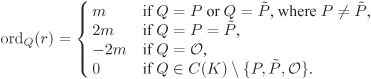
Example 2.23.

Let be a finite point on C. Consider the rational function , . The only points on C with X-coordinate equal to h are P and its opposite . Therefore, if P is an ordinary point, , whereas if P is a special point, ord_P (r) = 2m. Moreover, . For any , we have ord_Q(r) = 0.

Now consider r = (x – h)^m for some m < 0. Write r = G/H with G = 1 and H = (x – h)^–m. Since ord_Q(r) = ord_Q(G) – ord_Q(h), we continue to have

If m ≥ 0, then r is a polynomial function and has zeros P and and no finite poles. In this case, the sum of the orders of its zeros is 2m = 2 deg_x r = deg r. Theorem 2.52 generalizes this observation.

Theorem 2.52.

A non-constant polynomial function has only finitely many zeros and a single pole at . Furthermore, if K is algebraically closed, then .

2.12.3. The Jacobian

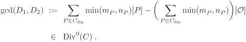
We continue to work with the hyperelliptic curve C of Equation (2.13). We first impose the restriction that K is algebraically closed and use the theory of Section 2.10 to define the set Div(C) of divisors on C, the degree zero part Div⁰(C) of Div(C), the divisor Div(r) of a rational function , the set Prin(C) of principal divisors on C, the Picard group Pic(C) = Div(C)/ Prin(C) and the Jacobian .

Example 2.24.

For the rational function r := (x – h)^m of Example 2.23, we have:

The Jacobian is the set of all cosets of Prin(C) in Div⁰(C). It is not a good idea to work with cosets (which are equivalence classes). Recall that in the case of , we represented a coset by the remainder of Euclidean division of a by n. In case of the representation , we took polynomials of smallest degrees as canonical representatives of the cosets of 〈f(X)〉. In case of too, we intend to find such good representatives, one from each coset. We now introduce the concept of reduced divisors for that purpose.

Definition 2.87.

Two divisors D₁, (resp. in Div(C)) are said to be equivalent, denoted D₁ ~ D₂, if , or equivalently if .

Our goal is to associate to every divisor some unique reduced divisor with D ~ D_red, that is, D_red plays the role of the canonical representative of . We start with the following definition.

Definition 2.88.

A divisor is called semi-reduced, if each m_P ≥ 0 and if for m_P > 0 we have: if P is an ordinary point, and m_P = 1 if P is a special point.

Proposition 2.41.

Every divisor is equivalent to some semi-reduced divisor D₁.

Proof

Let , with and with C_ord being the disjoint union of C₁ and C₂, where an ordinary point if and only if its opposite and . Now we can write D = D₁ + D₂, where

and

with m₁ and m₂ so chosen that D₁, . By definition, D₁ is semi-reduced, whereas by Example 2.24 , where

Now, we explain how we can represent a semi-reduced divisor by a pair of polynomials a(x), . For that, we need a definition.

Definition 2.89.

Let and be two divisors on C (not necessarily in Div⁰(P)). The greatest common divisor (gcd) of D₁ and D₂ is defined as the divisor

Theorem 2.53.

Let be a semi-reduced divisor on C. Let P_i = (h_i, k_i), i = 1, . . . , n, be the only finite points P on C such that m_P > 0. Let m_i := m_{P_i}, and (so that deg_x(a) = m). Then there exists a unique polynomial with the following properties:

deg_x b < m,
b(h_i) = k_i for i = 1, . . . , n,
a(x) divides b(x)² + b(x)u(x) – v(x), and
.

Conversely, if a(x), with deg_x b < deg_x a and with a dividing b² + bu – v, then the divisor gcd is semi-reduced.

We denote the divisor gcd by Div(a, b). The zero divisor has the representation Div(1, 0).

A representation of the elements of by semi-reduced divisors (that is, by pairs of polynomials in K[x]) suffers from two disadvantages. First, the representation is not unique, and second, the degrees of the representing polynomials may be quite large. These difficulties are removed if we consider semi-reduced divisors of a special kind.

Definition 2.90.

A semi-reduced divisor is called a reduced divisior, if , where g is the genus of C.

The following theorem establishes the desirable properties of a reduced divisor.

Theorem 2.54.

For , there exists a unique reduced divisor D₁ equivalent to D.

Proof

We only prove the existence of reduced divisors. For the proof of the uniqueness, one may, for example, see Koblitz [154]. The norm of a divisor is defined as the integer .

Let . By Proposition 2.41 there exists a semi-reduced divisor D′ ~ D. One can easily verify that |D′| ≤ |D|. If we already have |D′| ≤ g, then D′ is a desired reduced divisor. So assume otherwise, that is, |D′| ≥ g + 1. We can then choose finite points P₁, . . . , P_g+1 on C (not necessarily all distinct) such that is a subsum of the formal sum D′. Let the semi-reduced divisor be represented as Div(a, b) with deg_x a = g + 1 and deg_x b ≤ g. But then deg(b(x) – y) = 2g + 1 and b(x) – y has zeros at P₁, . . . , P_g+1 by Theorem 2.53. So by Theorem 2.52 we can write for some finite points Q₁, . . . , Q_g on C. Now satisfies D″ ~ D′ and |D″| < |D′|. We apply Proposition 2.41 again to get a semi-reduced divisor D‴ ~ D″ with |D‴| ≤ |D″|. Thus starting from the semi-reduced divisor D′ we produce another semi-reduced divisor D‴ such that D‴ ~ D′ ~ D and |D‴| < |D′|. We continue the process a finite number of times, until we get an equivalent semi-reduced divisor D₁ of norm ≤ g. This is a desired reduced divisor.

From the viewpoint of cryptography, the field K should be a finite field which is never algebraically closed. So we must remove the restriction . Since C is naturally defined over as well, we start with the Jacobian and define a particular subgroup of to be the Jacobian of C over K.

Definition 2.91.

Let be a K-automorphism of . For a point , the point is also in . For a divisor , we define . D is said to be defined over K if for all . The subset of consisting of divisor classes that have representative divisors defined over K is a subgroup (denoted by ) of and is called the Jacobian of C over K.

Every element of can be represented uniquely as a reduced divisor Div(a, b) for polynomials a(x), with deg_x a ≤ g and deg_x b < deg_x a. is, therefore, a finite Abelian group. For suitably chosen hyperelliptic curves, these groups can be used to build cryptographic protocols.

Exercise Set 2.12

In this exercise set, we let C denote a hyperelliptic curve of genus g defined by Equation (2.13) over a field K (not necessarily algebraically closed).

2.118	Show that the curve C₁ : Y² = X⁵ + X + 1 defined over is not smooth and so not a hyperelliptic curve. Find a point where C₁ is not smooth. Show that the curve C₂ : Y² = X⁵ + X + 2 defined over is smooth, that is, a hyperelliptic curve of genus 2. Find out all the -rational points on C₂. (There are ten of them.)
2.119	Represent as , where ξ is a root of the irreducible polynomial . Show that the curve C₃ : Y² + XY = X⁵ + X + 1 defined over is not smooth and so not a hyperelliptic curve. Find a point where C₃ is not smooth. Show that the curve C₄ : Y² + XY = X⁵ + X + ξ defined over is smooth, that is, a hyperelliptic curve of genus 2. Find out all the -rational points on C₄. (There are eight of them.)
2.120	Let . Prove the following assertions: The only points on C with X-coordinate equal to h are P and . . P is a special point if and only if u²(h) + 4v(h) = 0. If char K ≠ 2, then C has at most 2g + 1 special points, whereas if char K = 2, then C has at most g special points.
2.121	Prove Lemmas 2.9 and 2.10.
2.122	Let and . Show that G(P) = 0 if and only if . Let . Show that either P is a special point of C or h is a common root of u and v. Show that and that .
2.123	Prove Theorem 2.52. [H]
2.124	A line on C is a polynomial function of the form with a, b, , a and b not both 0. Let D = Div(l) be the divisor of a line l. Show that the norm \|D\| is either 2 or 2g + 1. Let . Determine Div(x – h). Determine Div(y).
2.125	Let E be an elliptic curve (that is, a hyperelliptic curve of genus 1) defined over K. Show that any divisor can be written as for some unique point and for some rational function . This rational function r is unique up to multiplication by elements of . Show that the map that maps the residue class of to the point satisfying for some , is a bijection. Let P, , not both . Show that there is a line l with , where R = –(P + Q). Let , where σ is defined in Part (b). Show that for P, one has . (This, in particular, proves Theorem 2.46 and that σ is a group isomorphism.) Let . Show that D is a principal divisor if and only if (integer sum) and (sum in ).