2.15. Statistical Methods

Many attacks on cryptosystems involve statistical analysis of ciphertexts and also of data collected from the victim’s machine during one or more private-key operations. For a proper understanding of these analysis techniques, one requires some knowledge of statistics and random variables. In this section, we provide a quick overview of some statistical gadgets. We make the assumption that the reader is already familiar with the elementary notion of probability. We denote the probability of an event E by Pr(E).

2.15.1. Random Variables and Their Probability Distributions

An experiment whose outcome is random is referred to as a random experiment. The set of all possible outcomes of a random experiment is called the sample space of the experiment. For example, the outcomes of tossing a coin can be mapped to the set {H, T} with H and T standing respectively for head and tail. It is convenient to assign numerical values to the outcomes of a random experiment. Identifying head with 0 and tail with 1, one can view coin tossing as a random experiment with sample space {0, 1}. Some other random experiments include throwing a die (with sample space {1, 2, 3, 4, 5, 6}), the life of an electric bulb (with sample space , the set of all non-negative real numbers), and so on. Unless otherwise specified, we henceforth assume that sample spaces are subsets of .

A random variable is a variable which can assume (all and only) the values from a (given) sample space.

A discrete random variable can assume only countably many values, that is, the sample space S_X of a discrete random variable X either is finite or has a bijection with , that is, we can enumerate the elements of S_X as x₁, x₂, x₃, . . ..

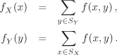
The probability distribution function or the probability mass function

f_X : S_X → [0, 1]

of a discrete random variable X assigns to each x in the sample space S_X of X the probability of the occurrence of the value x in a random experiment.^[21] We have

^[21] [a, b] is the closed interval consisting of all real numbers u satisfying a ≤ u ≤ b. Similarly, the open interval (a, b) is the set of all real values u satisfying a < u < b. In order to make a distinction between the open interval (a, b) and the ordered pair (a, b), many—mostly Europeans—use the notation ]a, b[ for denoting open intervals.

A continuous random variable assumes uncountable number of values, that is, the sample space S_X of a continuous random variable X cannot be in bijective correspondence with a subset of . Typically S_X is an interval [a, b] or (a, b) with –∞ ≤ a < b ≤ +∞.

One does not assign individual probabilities Pr(X = x) to a value assumed by a continuous random variable X.^[22] The probabilistic behaviour of X is in this case described by the probability density function

^[22] More correctly, Pr(X = x) = 0 for each .

with the implication that the probability that X occurs in the interval [c, d] (or (c, d)) is given by the integral

that is, by the area between the x-axis, the curve f_X(x) and the vertical lines x = c and x = d. We have

It is sometimes useful to set f_X(x) :=0 for , so that f_X is defined on the entire real line .

The cumulative probability distribution of a random variable X (discrete or continuous) is the function F_X (x) := Pr(X ≤ x) for all . If X is continuous, we have

which implies that

2.15.2. Operations on Random Variables

Let X and Y be discrete random variables. The joint probability distribution of X, Y refers to a random variable Z with S_Z = S_X × S_Y. For z = (x, y), the probability of Z = z is denoted by f_Z(z) = Pr(Z = z) = Pr(X = x, Y = y). The probability Pr(X = x, Y = y) stands for the probability that X = x and Y = y. The random variables X and Y are called independent, if

Pr(X = x, Y = y) = Pr(X = x) Pr(Y = y)

for all x, y.

Example 2.36.

Suppose that we have an urn containing three identical balls with labels 1, 2, 3. We draw two balls randomly from the urn. Let us denote the outcome of the first drawing by X and that of the second drawing by Y. We consider the joint distribution X, Y of the two outcomes in the two following cases: The balls are drawn with replacement, that is, after the first ball is drawn, it is returned back to the urn (and the urn is shaken well), before the next ball is drawn. The joint probability distribution is now as follows: In this case, the outcome of the second drawing is not influenced by the outcome of the first drawing; that is, X and Y are independent, and we have , as expected. The balls are drawn without replacement, that is, the ball obtained by the first drawing is not returned to the urn, before the second ball is drawn. In this case, the outcome of the second drawing is influenced by that of the first drawing in the sense that the same ball cannot be drawn on both occasions. Thus, X and Y are now dependent. This is revealed by the following joint probability distribution: x y Pr(X = x, Y = y) 1 1 0 1 2 1/6 1 3 1/6 2 1 1/6 2 2 0 2 3 1/6 3 1 1/6 3 2 1/6 3 3 0

For continuous random variables X and Y, the joint distribution is defined by the probability density function f_X,Y (x, y) and the cumulative distribution is obtained by the double integral

X and Y are independent, if f_X,Y (x, y) = f_X(x)f_Y (y) for all x, y. In this case, we also have F_X,Y (c, d) = F_X(c)F_Y (d) for all c, d.

Now, we define arithmetic operations on random variables. First, let X and Y be discrete random variables. The sum X + Y is defined to be a random variable U which assumes the values u = x + y for and with probability

The product XY of X and Y is defined to be a random variable V which assumes the values v = xy for and with probability

For , the random variable W = αX assumes the values w = αx for with probability

f_W(w) = Pr(W = αx) = Pr(X = x) = fX(x).

Example 2.37.

Let us consider the random variables X and Y of Example 2.36. For the sake of brevity, we denote Pr(X = x, Y = y) by Pxy. The distributions of U = X + Y in the two cases are as follows: Drawing with replacement: Pr(U = 2) = P11 = 1/9 Pr(U = 3) = P12 +P21 = 2/9 Pr(U = 4) = P13 +P22 + P31 = 1/3 Pr(U = 5) = P23 +P32 = 2/9 Pr(U = 6) = P33 = 1/9 Drawing without replacement: Pr(U = 3) = P12 +P21= 1/3 Pr(U = 4) = P13 +P31= 1/3 Pr(U = 5) = P23 +P32= 1/3

Now, let us consider continuous random variables X and Y. In this case, it is easier to define first the cumulative density functions of U = X + Y, V = XY and W = αX and then the probability density functions by taking derivatives:

One can easily generalize sums and products to an arbitrary finite number of random variables. More generally, if X₁, . . . , X_n are random variables and , one can talk about the probability distribution or density function of the random variable g(X₁, . . . , X_n). (See Exercise 2.163.)

Now, we introduce the important concept of conditional probability. Let X and Y be two random variables. To start with, suppose that they are discrete. We denote by f(x, y) = Pr(X = x, Y = y) the joint probability distribution function of X, Y. For with Pr(Y = y) > 0, we define the conditional probability of X = x given Y = y as:

For a fixed , the probabilities f_X|y(x), , constitute the probability distribution function of the random variable X|y (X given Y = y). If X and Y are independent, f(x, y) = f_X(x)f_Y (y) and so f_X|y(x) = f_X(x) for all , that is, the random variables X and X|y have the same probability distribution. This is expected, because in this case the probability of X = x does not depend on whatever value y the variable Y takes.

If X and Y are continuous random variables with joint density f(x, y) and , the conditional probability density function of X|y (X given Y = y) is defined by

Again if X and Y are independent, we have f_X|y(x) = f_X(x) for all x, y.

For a fixed , one can likewise define the conditional probabilities f_Y|x (y) := f(x, y)/f_X (x) for all .

Let X and Y be discrete random variables with joint distribution f(x, y). Also let Γ ⊆ S_X and Δ ⊆ S_Y. One defines the probability f_X(Γ) as:

The joint probability f(Γ, Δ), is defined as:

If Γ = {x} is a singleton, we prefer to write f(x, Δ) instead of f({x}, Δ). Similarly, f(Γ, y) stands for f (Γ,{y}). We also define the conditional distributions:

We abbreviate f_X|Δ (Γ) as Pr(Γ|Δ) and f_Y|Γ (Δ) as Pr(Δ|Γ).

Theorem 2.64. Bayes rule

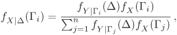
Let X, Y be discrete random variables and Δ ⊆ SY with fY (Δ) > 0. Also let Γ1,..., Γn form a partition of SX with fX (Γi) > 0 for all i = 1, . . . , n. Then we have: that is, in terms of probability: Proof Pr(Γi, Δ) = Pr(Δ|Γi) Pr(Γi) = Pr(Γi|Δ) Pr(Δ). So it is sufficient to show that Pr(Δ) equals the sum in the denominator. The event Δ is the union of the pairwise disjoint events (Γj, Δ), j = 1,..., n, and so .

The Bayes rule relates the a priori probabilities Pr(Γ_j) and Pr(Δ|Γ_j) to the a posteriori probabilities Pr(Γ_i|Δ). The following example demonstrates this terminology.

Example 2.38.

Consider the random experiment of Example 2.36(2). Take Γj := {j} for and Δ := {2, 3}. We have the following a priori probabilities: Pr(Γj) = Probability of getting ball j in the first draw = 1/3, Pr(Δ|Γ1) = Probability of getting the second or the third ball in the second draw, given that the first ball is obtained in the first draw = 1, Pr(Δ|Γ2) = Probability of getting the second or the third ball in the second draw, given that the second ball is obtained in the first draw = 1/2, Pr(Δ|Γ3) = Probability of getting the second or the third ball in the second draw, given that the third ball is obtained in the first draw = 1/2. 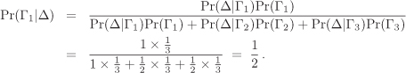The a posteriori probability Pr(Γ1|Δ) that the first ball was obtained in the first draw given that the ball obtained in the second draw is the second or the third one is calculated using the Bayes rule as: One can similarly calculate . This is expected, since the only events (x, y) consistent with are the four equiprobable possibilities (1, 2), (1, 3), (2, 3) and (3, 2).

2.15.3. Expectation, Variance and Correlation

Let X be a random variable. The expectation E(X) of X is defined as follows:

E(X) is also called the (arithmetic) mean or average of X. One uses the alternative symbols μ_X and to denote E(X). More generally, let X₁, . . . , X_n be n random variables with joint probability distribution/density function f(x₁, . . . , x_n). Also let . We define the following expectations:

X is discrete:

X is continuous:

Let g(X) and h(Y) be real polynomial functions of the random variables X and Y and let . Then

E(g(X) + h(Y))	=	E(g(X)) + E(h(Y)),
E(g(X)h(Y))	=	E(g(X)) E(h(Y)) if X and Y are independent,
E(αg(X))	=	αE(g(X)).

Let us derive the sum and product formulas for discrete variables X and Y.

If X and Y are independent, then

The variance Var(X) of a random variable X is defined as

Var (X) := E[(X – E(X))²].

From the observation that E[(X – E(X))²] = E[X² – 2 E(X)X + [E(X)]²] = E(X²) – 2 E(X) E(X) + [E(X)]², we derive the computational formula:

Var (X) = E[X²] – [E(X)]².

Var(X) is a measure of how the values of X are dispersed about the mean E(X) and is always a non-negative quantity. The (non-negative) square root of Var(X) is called the standard deviation σ_X of X:

The following formulas can be easily verified:

Var(X + α)	=	Var(X).
Var(αX)	=	α2 Var(X).
Var(X + Y)	=	Var(X) + Var(Y) + 2 Cov(X, Y),

where and where the covariance Cov(X, Y) of X and Y is defined as:

Cov(X, Y) := E[(X – E(X))(Y – E(Y))] = E(XY) – E(X) E(Y).

Normalized covariance is a measure of correlation between the two random variables X and Y. More precisely, the correlation coefficient ρ_X,Y is defined as:

If X and Y are independent, E(XY) = E(X) E(Y) so that Cov(X, Y) = 0 and so ρ_X,Y = 0. The converse of this is, however, not true, that is, ρ_X,Y = 0 does not necessarily imply that X and Y are independent. ρ_X,Y is a real value in the interval [–1, 1] and is a measure of linear relationship between X and Y. If larger (resp. smaller) values of X are (in general) associated with larger (resp. smaller) values of Y, then ρ_X,Y is positive. On the other hand, if larger (resp. smaller) values of X are (in general) associated with smaller (resp. larger) values of Y, then ρ_X,Y is negative.

Example 2.39.

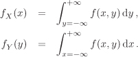
Once again consider the drawing of two balls from an urn containing three balls labelled {1, 2, 3} (Examples 2.36, 2.37 and 2.38). Look at the second case (drawing without replacement). We use the shorthand notation Pxy for Pr(X = x, Y = y). The individual probability distributions of X and Y can be obtained from the joint distribution as follows: Pr(X = 1) = P11 + P12 + P13 = 0 + (1/6) + (1/6) = 1/3 Pr(X = 2) = P21 + P22 + P23 = (1/6) + 0 + (1/6) = 1/3 Pr(X = 3) = P31 + P32 + P33 = (1/6) + (1/6) + 0 = 1/3         Pr(Y = 1) = P11 + P21 + P31 = 0 + (1/6) + (1/6) = 1/3 Pr(Y = 2) = P12 + P22 + P32 = (1/6) + 0 + (1/6) = 1/3 Pr(Y = 3) = P13 + P23 + P33 = (1/6) + (1/6) + 0 = 1/3 Thus E(X) = 1 × (1/3) + 2 × (1/3) + 3 × (1/3) = 2. Similarly, E(Y) = 2. Therefore, E(X + Y) = E(X) + E(Y) = 4. This can also be verified by direct calculations: E(X + Y) = 3 × (1/3) + 4 × (1/3) + 5 × (1/3) = 4. E(X2) = E(Y2) = 12 × (1/3) + 22 × (1/3) + 32 × (1/3) = 14/3 and Var(X) = Var(Y) = (14/3) – 22 = 2/3. The probability distribution for XY is E(XY = 2) = P12 + P21 = 1/3 E(XY = 3) = P13 + P31 = 1/3 E(XY = 6) = P23 + P32 = 1/3, so that E(XY) = 2 × (1/3) + 3 × (1/3) + 6 × (1/3) = 11/3. Therefore, Cov(XY) = E(XY) – E(X) E(Y) = (11/3) – 2 × 2 = –1/3, that is, The negative correlation between X and Y is expected. If X = 1 (small), Y takes bigger values (2, 3). On the other hand, if X = 3 (large), Y assumes smaller values (1, 2). Of course, the correlation is not perfect, since for X = 2 the values of Y can be smaller (1) or larger (3). So, we should feel happy to see a not-so-negative correlation of –1/2 between X and Y.

2.15.4. Some Famous Probability Distributions

Some probability distributions that occur frequently in statistical theory and in practice are described now. Some other useful probability distributions are considered in the Exercises 2.169, 2.170 and 2.171.

Uniform distribution

A discrete uniform random variable U has sample space S_U := {x₁, . . . , x_n} and probability distribution

A continuous uniform random variable U has sample space S_U and probability density function

where A > 0 is the size^[23] of S_U. For example, if S_U is the real interval [a, b] for a < b, we have

^[23] If , “size” means length. If or , “size” refers to area or volume respectively. We assume that the size of S_U is “measurable”.

In this case, we have

E(U) = (a + b)/2

and

Var(U) = (b – a)2/12.

Uniform random variables often occur naturally. For example, if we throw an unbiased die, the six possible outcomes (1 through 6) are equally likely, that is, each possible outcome has the probability 1/6. Similarly, if a real number is chosen randomly in the interval [0, 1], we have a continuous uniform random variable. The built-in C library call rand() (pretends to) return an integer between 0 and 2³¹ – 1, each with equal probability (namely, 2^–31).

Bernoulli distribution

The Bernoulli random variable B = B(n, p) is a discrete random variable characterized by two parameters and , where p stands for the probability of a certain event E and n represents the number of (independent) trials. It is assumed that the probability of E remains constant (namely, p) in each of the n trials. The sample space S_B = {0, 1, . . . , n} comprises the (exact) numbers of occurrences of E in the n trials. B has the probability distribution

as follows from simple combinatorial arguments. The mean and variance of B are:

E(B) = np

and

Var(B) = np(1 – p).

The Bernoulli distribution is also called the binomial distribution.

Normal distribution

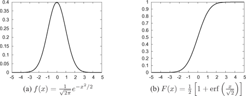
The normal random variable or the Gaussian random variable N = N (μ, σ²) is a continuous random variable characterized by two real parameters μ and σ with σ > 0. The density function of N is

The cumulative distribution for N can be expressed in terms of the error function erf():

The error function does not have a known closed-form expression. Figure 2.3 shows the curves for f_N (x) and F_N (x) for the parameter values μ = 0 and σ = 1 (in this case, N is called the standard normal variable).

Some statistical properties of N are:

E(N) = μ

and

Var(N) = σ2.

The curve f_N (x) is symmetric about x = μ. Most of the area under the curve is concentrated in the region μ – 3σ ≤ x ≤ μ + 3σ. More precisely:

Pr(μ – σ ≤ X ≤ μ + σ)	≈	0.68,
Pr(μ – 2σ ≤ X ≤ μ + 2σ)	≈	0.95,
Pr(μ – 3σ ≤ X ≤ μ + 3σ)	≈	0.997.

Many distributions occurring in practice (and in nature) approximately follow normal distributions. For example, the height of (adult) people in a given community is roughly normally distributed. Of course, the height of a person cannot be negative, whereas a normal random variable may assume negative values. But, in practice, the probability that such an approximating normal variable assumes a negative value is typically negligibly low.

2.15.5. Sample Mean, Variation and Correlation

In practice, we often do not know a priori the probability distribution or density function of a random variable X. In some cases, we do not have the complete data, whereas in some other cases we need an infinite amount of data to obtain the actual probability distribution of a random variable. For example, let X represent the life of an electric bulb manufactured by a given company in the last ten years. Even though there are only finitely many such bulbs and even if we assume that it is possible to trace the working of every such bulb, we have to wait until all these bulbs burn out, before we know the actual distribution of X. That is certainly impractical. On the contrary, if we have data on the life-times of some sample bulbs, we can approximate the properties of X by those of the samples.

Suppose that S := (x₁, x₂, . . . , x_n) is a sample of size n. We assume that all x_i are real numbers. We define the following quantities for S:

Here is the mean of the collection .

If T := (y₁, y₂, . . . , y_m) is another sample (of real numbers), the (linear) relationship between S and T is measured by the following quantities:

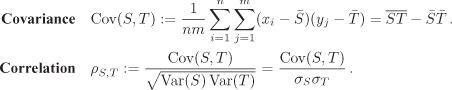
Here is the mean of the collection ST := (x_iy_j | i = 1, . . . , n, j = 1, . . . , m).

An important property of the normal distribution is the following:

Theorem 2.65. Central limit theorem

Let X be any random variable with mean μ and variance σ2 and let . The mean of a random sample S of size n chosen according to the distribution of X approximately follows the normal distribution N (μ, σ2/n). The larger the sample size n is, the better this approximation is.

Exercise Set 2.15

2.162	An urn contains n1 red balls and n2 black balls. We draw k balls sequentially and randomly from the urn, where 1 ≤ k ≤ n1 + n2. If the balls are drawn with replacement, what is the probability that the k-th ball drawn from the urn is red? If the balls are drawn without replacement, what is the probability that the k-th ball drawn from the urn is red?
2.163	Let X and Y be the random variables of Example 2.36. For each of the two cases, calculate the probability distribution functions, expectations and variances of the following random variables: XY 2X + 3Y X2 X2 + 2XY + Y2 (X + Y)2
2.164	Let X and Y be continuous random variables, g(X) and h(Y) non-constant real polynomials and α, β, . Prove that: E(g(X) + h(Y)) = E(g(X)) + E(h(Y)). E(g(X)h(Y)) = E(g(X)) E(h(Y)), if X and Y are independent. E(αg(X)) = αE(g(X)). Var(αX + βY + γ) = α2 Var(X) + β2 Var(Y).
2.165	Let X be a random variable and Y := αX + β for some α, . What is ρX,Y ?
2.166	Let X and Y be discrete random variables with joint probability distribution function f(x, y). Show that the probability distributions of X and Y can be obtained as If X and Y are continuous random variables with joint density function f(x, y), show that the density functions of X and Y are given by The functions fX and fY are called the marginal probability distribution (or density function) of X and Y respectively.
2.167	Let X and Y be continuous random variables whose joint distribution is the uniform distribution in the triangle 0 ≤ X ≤ Y ≤ 1. Compute the marginal distributions fX and fY. Compute E(X), E(Y), Var(X), Var(Y), Cov(X, Y) and ρX,Y.
2.168	Let X, Y, Z be random variables. Show that: Cov(X, Y) = Cov(Y, X). ρX,Y = ρY,X. Cov(X, X) = Var(X). Cov(X, Y + Z) = Cov(X, Y) + Cov(X, Z). Cov(X, X + Y) = Var(X) + Cov(X, Y). Cov(X, X + Y) = Var(X) if X and Y are independent.
2.169	Geometric distribution Assume that in each trial of an experiment, an event E has a constant probability p of occurrence. Let G = G(p) denote the random variable with and with fG(x) equal to the probability that E occurs the first time during the x-th trial (that is, after exactly x – 1 failures). Show that: What if p = 0?
2.170	Poisson distribution Let P = P (λ) be the discrete random variable with and with , where λ is a positive real constant. Show that E(P) = Var(P) = λ.
2.171	Exponential distribution Let X = X(λ) be the continuous random variable with density where λ is a positive real constant. Show that: A random variable Y with is said to be memoryless, if Pr(Y > s + t | Y > s) = Pr(Y > t) for all s, . Show that the exponential variable X of Part (a) is memoryless.
2.172	The birthday paradox Let S be a finite set of cardinality n. Show that the probability that k < n elements, drawn at random form S (with replacement), are (pairwise) distinct is Use the inequality 1 – x ≤ e–x for any real number x to show that . Deduce that p ≤ 1/2, if , and that p ≤ 0.136 for . (The birthday paradox states that if only 23 people are chosen at random, there is a chance as high as 50 per cent that at least two of them have the same birthday.)