4.3. The Integer Factorization Problem

The integer factorization problem (IFP) (Problems 4.1, 4.2 and 4.3) is one of the most easily stated and yet hopelessly difficult computational problem that has attracted researchers’ attention for ages and most notably in the age of electronic computers. A huge number of algorithms varying widely in the basic strategy, mathematical sophistication and implementation intricacy have been suggested, and, in spite of these, factoring a general integer having only 1000 bits seems to be an impossible task today even using the fastest computers on earth.

It is important to note here that even proving rigorous bounds on the running times of the integer-factoring algorithms is quite often a very difficult task. In many cases, we have to be satisfied with clever heuristic bounds based on one or more reasonable but unprovable assumptions.

This section highlights human achievements in the battle against the IFP. Before going into the details of this account we want to mention some relevant points. Throughout this section we assume that we want to factor a (positive) integer n. Since such an integer can be represented by ⌈lg(n + 1)⌉ bits, the input size is taken to be lg n (or, ln n, or log n). Most modern factorization algorithms take time given by the following subexponential expression in ln n:

L(n, α, c) := exp((c + o(1))(ln n)^α(ln ln n)^1–α),

where 0 < α < 1 and c > 0 are constants. As described in Section 3.2, the smaller the value of α is, the closer the expression L(n, α, c) is to a polynomial expression (in ln n). If n is understood from the context, we write L(α, c) in place of L(n, α, c). Although the current best-known algorithms correspond to α = 1/3, the algorithms with α = 1/2 are also quite interesting. In this case, we use the shorter notation L[c] := L(1/2, c).

Henceforth we will use, without explicit mention, the notation q₁ := 2, q₂ := 3, q₃ := 5, . . . to denote the sequence of primes. The concept of q_t-smoothness (for some ) will often be referred to as B-smoothness, where B = {q₁, . . . , q_t}. Recall from Theorem 2.21 that smaller integers have higher probability of being B-smooth for a given B. This observation plays an important role in designing integer factoring algorithms. The following special case of Theorem 2.21 is often useful.

Corollary 4.1.

Let , x = O(nα) and y = L[β] = L(n, 1/2, β). Then we have the asymptotic formula . Before any attempt of factoring n is made, it is worthwhile to check for the primality of n. Since probabilistic primality tests (like Algorithm 3.13) are quite efficient, we should first run one such test before we are sure that n is really composite. Henceforth, we will assume that n is known to be composite.

4.3.1. Older Algorithms

“Factoring in the dark ages” (a phrase attributed to Hendrik Lenstra) used fully exponential algorithms some of which are discussed now. Though the worst-case performances of these algorithms are quite poor, there are many situations when they might factor even a large integer quite fast. It is, therefore, worthwhile to spend some time on these algorithms.

Trial division

A composite integer n admits a factor ≤ , that can be found by trial divisions of n by integers ≤ . This demands trial divisions and is clearly impractical, even when n contains only 30 decimal digits. It is also true that n has a prime divisor ≤ . So it suffices to carry out trial divisions by primes only. Though this modified strategy saves us many unnecessary divisions, the asymptotic complexity does not reduce much, since by the prime number theorem the number of primes ≤ is about . In addition, we need to have a list of primes ≤ or generate the primes on the fly, neither of which is really practical. A trade-off can be made by noting that an integer m ≥ 30 cannot be prime unless m ≡ 1, 7, 11, 13, 17, 19, 23, 29 (mod 30). This means that we need to perform the trial divisions only by those integers m congruent to one of these values modulo 30 and this reduces the number of trial divisions to about 25 per cent. Though trial division is not a practical general-purpose algorithm for factoring large integers, we recommend extracting all the small prime factors of n, if any, by dividing n by a predetermined set {q₁, . . . , q_t} of small primes. If n is indeed q_t-smooth or has all prime factors ≤ q_t except only one, then the trial division method completely factors n quite fast. Even when n is not of this type, trial division might reduce its size, so that other algorithms run somewhat more efficiently.

Pollard’s rho method

Pollard’s rho method solves the IFP in an expected O^~(n^1/4) time and is based on the birthday paradox (Exercise 2.172).

Let be an (unknown) prime divisor of n and let be a random map. We start with an initial value and generate a sequence x_i+1 = f(x_i), , of elements of . Let y_i denote the smallest non-negative integer satisfying y_i ≡ x_i (mod p). By the birthday paradox, after iterates x₁, . . . , x_t are generated, we have a high chance that y_i = y_j, that is, x_i ≡ x_j (mod p) for some 1 ≤ i < j ≤ t. This means that p|(x_i – x_j) and computing gcd(x_i – x_j, n) splits n into two non-trivial factors with high probability. The method fails if this gcd is n. For a random n, this incident of having a gcd equal to n is of very low probability.

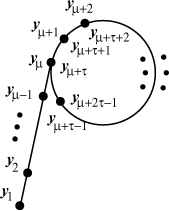
Algorithm 4.1 gives a specific implementation of this method. Computing gcds for all the pairs (x_i – x_j, n) is a massive investment of time. Instead we store (in the variable ξ) the values x_r, r = 2^t, for and compute only gcd(x_r+s – x_r, n) for s = 1, . . . , r. Since the sequence y_i, , is ultimately periodic with expected length of period , we eventually reach a t with r = 2^t ≥ τ. In that case, the for loop detects a match. Typically, the update function f is taken to be f(x) = x² –1 (mod n), which, though not a random function, behaves like one. Note that the iterates y_i, , may be visualized as being located on the Greek letter ρ as shown in Figure 4.1 (with a tail of the first μ iterates followed by a cycle of length τ). This is how this method derives its name.

Algorithm 4.1 takes an expected running time . Since , Pollard’s rho method runs in expected time .

Algorithm 4.1. Pollard’s rho method

Input: A composite integer . Output: A non-trivial factor of n. Steps: Choose a random element and set ξ := x and r := 1. while (1) {    for s = 1, . . . , r {        x := f(x).        d := gcd(x – ξ, n).        if (1 < d < n) { Return d. }    }    ξ := x.    r := 2r. }

Many modifications of Pollard’s rho method have been proposed in the literature. Perhaps the most notable one is an idea due to R. P. Brent. All these modifications considerably speed up Algorithm 4.1, though leaving the complexity essentially the same, that is, . We will not describe these modifications in this book.

Pollard’s p – 1 method

Pollard’s p – 1 method is dependent on the prime factors of p – 1 for a prime divisor p of n. Indeed if p – 1 is rather smooth, this method may extract a (non-trivial) factor of n pretty fast, even when p itself is quite large. To start with we extend the definition of smoothness as follows.

Definition 4.1.

Let . An integer x is called y-power-smooth if, whenever a prime power pe divides x, we have pe ≤ y. Clearly, a y-power-smooth integer is y-smooth, but not necessarily conversely.

Let p be an (unknown) prime divisor of n. We may assume, without loss of generality, that . Assume that p–1 is M-power-smooth. Then (p – 1)| lcm(1, . . . , M) and, therefore, for an integer a with gcd(a, n) = 1 (and hence with gcd(a, p) = 1), we have a^lcm(1,...,M) ≡ 1 (mod p) by Fermat’s little theorem, that is, d := gcd(a^lcm(1,...,M) – 1, n) > 1. If d ≠ n, then d is a non-trivial factor of n. In case we have d = n (a very rare occurrence), we may try with another a or declare failure.

The problem with this method is that p and so M are not known in advance. One may proceed by guessing successively increasing values of M, till the method succeeds. In the worst case, that is, when p is a safe prime, we have M = (p – 1)/2. Since , this algorithm runs in a worst-case time of . However, if M is quite small, then this algorithm is rather efficient, irrespective of how large p itself is.

In Algorithm 4.2, we give a variant of the p – 1 method, where we supply a predetermined value of the bound M. We also assume that we have at our disposal a precalculated list of all primes q₁, . . . , q_t ≤ M.

There is a modification of this algorithm known as Stage 2 or the second stage. For this, we choose a second bound M′ larger than M. Assume that p – 1 = rq, where r is M-power-smooth and q is a prime in the range M < q ≤ M′. In this case, Stage 2 computes with high probability a factor of n after doing an operations as follows. When Algorithm 4.2 returns “failure” at the last step, it has already computed the value A := a^m (mod n), where , e_i = ⌊ln M/ln q_i⌋. In this case, A has the multiplicative order of q modulo p, that is, the subgroup H of generated by A has order q. We choose random integers . By the birthday paradox (Exercise 2.172), we have with high probability A^l_i ≡ A^l_j (mod p) for some i ≠ j. In that case, d := gcd(A^l_i – A^l_j, n) is divisible by p and is a desired factor of n (unless d = n, a case that occurs with a very low probability). In practice, we do not know q and so we determine s and the integers l₁, . . . , l_s using the bound M′ instead of q.

Algorithm 4.2. Pollard’s p – 1 method

Input: A composite integer , a bound M and all primes q1, . . . , qt ≤ M. Output: A non-trivial factor d of n or “failure”. Steps: Select a random integer a, 1 < a < n. /* For example, we may take a := 2 */ if (d := gcd(a, n) ≠ 1) { Return d. } for i = 1, . . . , t {     ei := ⌊ln M/ln qi⌋.     .     d := gcd(a – 1, n)     if (1 < d < n) { Return d. }     if (d = n) { Return “failure”. }  /* Or repeat the for loop with another a */     if (d = 1) { Return “failure”. } } Return “failure”.

In another variant of Stage 2, we compute the powers A^q_t+1 , . . . , A^q_t′ (mod n), where q_t+1, . . . , q_t′ are all the primes q_j satisfying M < q_j ≤ M′. If p – 1 = rq is of the desired form, we would find q = q_j for some t < j ≤ t′, and then gcd(A^q – 1, n), if not equal to n, would be a non-trivial factor of n.

In practice, one may try one’s luck using this algorithm for some M in the range 10⁵ ≤ M ≤ 10⁶ (and possibly also the second stage with 10⁶ ≤ M′ ≤ 10⁸) before attempting a more sophisticated algorithm like the MPQSM, the ECM or the NFSM.

Williams’ p + 1 method

As always, we assume that n is a composite integer and that p is an (unknown) prime divisor of n. Pollard’s p – 1 method uses an element a in the group whose multiplicative order is p – 1. The idea of Williams’ p + 1 method is very similar, that is, it works with an element a, this time in , whose multiplicative order is p + 1. If p + 1 is M-power-smooth for a reasonably small bound M, then computing d := gcd(a^p+1 – 1, n) > 1 splits n with high probability.

In order to find an element of order p + 1, we proceed as follows. Let α be an integer such that α² – 4 is a quadratic non-residue modulo p. Then the polynomial is irreducible and . Let a, be the two roots of f. Then ab = 1 and a + b = α. Since f(a^p) = 0 (check it!) and since , we have a^p = b = a^–1, that is, a^p+1 = 1.

Unfortunately, p is not known in advance. Therefore, we represent elements of as integers modulo n and the elements of as polynomials c₀ + c₁X with c₀, . Multiplying two such elements of is accomplished by multiplying the two polynomials representing these elements modulo the defining polynomial f(X), the coefficient arithmetic being that of . This gives us a way to do exponentiations in in order to compute a^m – 1 for a suitable m (for example, m = lcm(1, . . . , M)).

However, the absence of knowledge of p has a graver consequence, namely, it is impossible to decide whether α² – 4 is a quadratic non-residue modulo p for a given integer α. The only thing we can do is to try several random values of α. This is justified, because if k random integers α are tried, then the probability that for all of these α the integers α² – 4 are quadratic residues modulo p is only 1/2^k.

The code for the p + 1 method is very similar to Algorithm 4.2. We urge the reader to complete the details. Since p³ – 1 = (p – 1)(p² + p + 1), p⁴ – 1 = (p² – 1)(p² + 1) and so on, we can work in higher extensions like , to find elements of order p² + p + 1, p² + 1 and so on, and generalize the p ± 1 methods. However, the integers p² + p + 1, p² + 1, being large (compared to p ± 1), have smaller chance of being M-smooth (or M-power-smooth) for a given bound M.

The reader should have recognized why we paid attention to strong primes and safe primes (Definition 3.5, p 199, and Algorithm 3.14, p 200). Let us now concentrate on the recent developments in the IFP arena.

4.3.2. The Quadratic Sieve Method

Carl Pomerance’s quadratic sieve method (QSM) is one of the (reasonably) successful modern methods of factoring integers. Though the number field sieve factoring method is the current champion, there was a time in the recent past when the quadratic sieve method and the elliptic curve method were known to be the fastest algorithms for solving the IFP.

The basic algorithm

We assume that n is a composite integer which is not a perfect square (because it is easy to detect if n is a perfect square and if so, we replace n by ). The basic idea is to reach at a congruence of the form

Equation 4.1

with x ≢ ±y (mod n). In that case, gcd(x – y, n) is a non-trivial factor of n.

We start with a factor base B = {q₁, . . . , q_t} comprising the first t primes and let and J := H² – n. Then H and J are each and hence for a small integer c the right side of the congruence

(H + c)² ≡ J + 2cH + c² (mod n)

is also . We try to factor T(c) := J + 2cH + c² using trial divisions by elements of B. If the factorization is successful, that is, if T(c) is B-smooth, then we get a relation of the form

Equation 4.2

where . (Note that T(c) ≠ 0, since n is assumed not to be a perfect square.) If all α_i are even, say, α_i = 2β_i, then we get the desired Congruence (4.1) with and y = H + c. But this is rarely the case. So we keep on generating other relations. After sufficiently many relations are available, we combine these together (by multiplication) to get Congruence (4.1) and compute gcd(x – y, n). If this does not give a non-trivial factor, we try to recombine the collected relations in order to get another Congruence (4.1). This is how Pomerance’s QSM works.

In order to find suitable combinations for yielding Congruence (4.1), we employ a method similar to Gaussian elimination. Assume that we have collected r relations of the form

We search for integers such that the product

is a desired Congruence (4.1). The left side of this congruence is already a square. In order to make the right side a square too, we have to essentially solve the following system of linear congruences modulo 2:

This is a system of t equations over in r unknowns β₁, . . . , β_r and is expected to have solutions, if r is slightly larger than t. Note that the values of α_ij modulo 2 are only needed for solving the above linear system. This means that we can have a compact representation of the coefficient matrix (α_ij) by packing 32 of the coefficients as bits per word. Gaussian elimination (over ) can be done using bit operations only.

The running time of this method can be derived using Corollary 4.1. Note that the integers T(c) that are tested for B-smoothness are O(n^1/2) which corresponds to α = 1/2 in the corollary. We take q_t = L[1/2] (so that t = L[1/2]/ ln L[1/2] = L[1/2] by the prime number theorem) which corresponds to β = 1/2. Assuming that the integers T(c) behave as random integers of magnitude O(n^1/2), the probability that one such T(c) is B-smooth is L[–1/2]. Therefore, if L[1] values of c are tried, we expect to get L[1/2] relations involving the L[1/2] primes q₁, . . . , q_t. Combining these relations by Gaussian elimination is now expected to produce a non-trivial Congruence (4.1). This gives us a running-time of the order of L[3/2] for the relation collection stage. Gaussian elimination using L[1/2] unknowns also takes asymptotically the same time. However, each T(c) can have at most O(log n) distinct prime factors, implying that Relation (4.2) is necessarily sparse. This sparsity can be effectively exploited and the Gaussian elimination can be done essentially in time L[1]. Nevertheless, the entire procedure runs in time L[3/2], a subexponential expression in ln n.

Sieving

In order to reduce the running time from L[3/2] to L[1], we employ what is known as sieving (and from which the algorithm derives its name). Let us fix a priori the sieving interval, that is, the values of c for which T(c) is tested for B-smoothness, to be –M ≤ c ≤ M, where M = L[1]. Let be a small prime (that is, q = q_i for some i = 1, . . . , t). We intend to find out the values of c such that q^h|T(c) for small exponents h = 1, 2, . . . . Since T(c) = J + 2cH + c² = (c + H)² – n, the solvability for c of the condition q^h|T(c) or of q|T(c) is equivalent to the solvability of the congruence (c + H)² ≡ n (mod q). If n is a quadratic non-residue modulo q, no c satisfies the above condition. Consequently, the factor base B may comprise only those primes q for which n is a quadratic residue modulo q (instead of all primes ≤ q_t). So we assume that q meets this condition. We may also assume that q  n, because it is a good strategy to perform trial divisions of n by all the primes in B before we go for sieving. The sieving process makes use of an array indexed by c. We initialize the array location for each c, –M ≤ c ≤ M.

We explain the sieving process only for an odd prime q. The modifications for the case q = 2 are left to the reader as an easy exercise. The congruence x² – n ≡ 0 (mod q) has two distinct solutions for x, say, x₁ and mod q. These correspond to two solutions for c of (H + c)² ≡ n (mod q), namely, c₁ ≡ x₁ – H (mod q) and (mod q). For each value of c in the interval –M ≤ c ≤ M, that is congruent either to c₁ or modulo q, we subtract ln q from . We then lift the solutions x₁ and to the (unique) solutions x₂ and of the congruence x² – n ≡ 0 (mod q²) (Exercise 3.29), compute c₂ ≡ x₂ – H (mod q²) and (mod q²) and for each c in the range –M ≤ c ≤ M congruent to c₂ or modulo q² subtract ln q from . We then again lift to obtain the solutions modulo q³ and proceed as above. We repeat this process of lifting and subtracting ln q from appropriate locations of until we reach a sufficiently large for which neither c_h nor corresponds to any value of c in the range –M ≤ c ≤ M. We then choose another q from the factor base and repeat the procedure explained in this paragraph for this q.

After the sieving procedure is carried out for all small primes q in the factor base B, we check for which c, –M ≤ c ≤ M, the array location is 0. These are precisely the values of c in the indicated range for which T(c) is B-smooth. For each smooth T(c), we then compute Relation (4.2) using trial division (by primes of B).

The sieving process replaces trial divisions (of every T(c) by every q) by subtractions (of ln q from appropriate ). This is intuitively the reason why sieving speeds up the relation collection stage. For a more rigorous analysis of the running time, note that in order to get the desired c_i and modulo qⁱ for each and for each i = 1, . . . , h we have either to compute a square root modulo q (for i = 1) or to solve a congruence (during lifting for i ≥ 2), each of which can be done in polynomial time. Also the bound h on the exponent of q satisfy , that is, h = O(log n). Finally, there are L[1/2] primes in B. Therefore, the computation of the c_i and for all q and i takes a total of L[1/2] time.

Now, we count the total number ν of subtractions of different ln q values from all the locations of the array . The size of is 2M + 1. For each qⁱ, we need to subtract ln q from at most 2 ⌈(2M + 1)/qⁱ⌉ locations (for odd q), and we also have . Therefore, ν is of the order of , where Q is the maximum of all qⁱ and is , and where H_m, , denote the harmonic numbers (Exercise 4.6). But H_m = O(ln m), and so ν = O(2(2M + 1) log n) = L[1], since M = L[1].

The logarithms ln q (as well as the initial array values ln |T(c)|) are irrational numbers and hence need infinite precision for storing. We, however, need to work with only crude approximations of these logarithms, say up to three places after the decimal point. In that case, we cannot take as the criterion for selecting smooth values of T(c), because the approximate representation of logarithms leads to truncation (and/or rounding) errors. In practice, this is not a severe problem, because T(c) is not smooth if and only if it has a prime factor at least as large as q_t+1 (the smallest prime not in B). This implies that at the end of the sieving operation the values of for smooth T(c) are close to 0, whereas those for non-smooth T(c) are much larger (close to a number at least as large as ln q_t+1). Thus we may set the selection criterion for smooth integers as or as ln q_t+1. It is also possible to replace floating point subtraction by integer subtraction by doing the arithmetic on 1000 times the logarithm values. To sum up, the ν = L[1] subtractions the sieving procedure does would be only single-precision operations and hence take a total of L[1] time.

As mentioned earlier, Gaussian elimination with sparse equations can also be performed in time L[1]. So Pomerance’s algorithm with sieving takes time L[1].

Incomplete sieving

Numerous modifications over this basic strategy speed up the algorithm reasonably. One possibility is to do sieving every time only for h = 1 and ignore all higher powers of q. That is, for every q we check which of the integers T(c) are divisible by q and then subtract ln q from the corresponding indices of the array . If some T(c) is divisible by a higher power of q, this strategy fails to subtract ln q the required number of times. As a result, this T(c), even if smooth, may fail to pass the smoothness criterion. This problem can be overcome by increasing the cut-off from 1 (or 0.1 ln q_t+1) to a value ξ ln q_t for some ξ ≥ 1. But then some non-smooth T(c) will pass through the selection criterion in addition to some smooth ones that could not, otherwise, be detected. This is reasonable, because the non-smooth ones can be later filtered out from the smooth ones and one might use even trial divisions to do so. Experimentations show that values of ξ ≤ 2.5 work quite well in practice.

The reason why this strategy performs well is as follows. If q is small, for example q = 2, we should subtract only 0.693 from for every power of 2 dividing T(c). On the other hand, if q is much larger, say q = 1,299,709 (the 10⁵-th prime), then ln q ≈ 14.078 is large. But T(c) would not, in general, be divisible by a high power of this q. This modification, therefore, leads to a situation where the probability that a smooth T(c) is actually detected as smooth is quite high. A few relations would still be missed out even with the modified selection criterion, but that is more than compensated by the speed-up gained by the method. Henceforth, we will call this modified strategy as incomplete sieving and the original strategy (of considering all powers of q) as complete sieving.

Large prime variation

Another trick known as large prime variation also tends to give more usable relations than are available from the original (complete or incomplete) sieving. In this context, we call a prime q′ large, if q′ ∉ B. A value of T(c) is often expected to be B-smooth except for a single large prime factor:

Equation 4.3

with q′ ∉ B. Such a value of T(c) can be easily detected. For example, incomplete sieving with the relaxed selection criterion is expected to give many such relations naturally, whereas for complete sieving, if the left-over of ln |T(c)| in at the end of the subtraction steps is < 2 ln q_t, then this must correspond to a large prime factor < . Instead of throwing away an apparently unusable Equation (4.3), we may keep track of them. If a large prime q′ is not large enough (that is, not much larger than q_t), then it might appear on the right side of Equation (4.3) for more than one values of c, and if that is the case, all these relations taken together now become usable for the subsequent Gaussian elimination stage (after including q′ in the factor base). This means that for each large prime occurring more frequently than once, the factor base size increases by 1, whereas the number of relations increases by at least 2. Thus with a little additional effort we enrich the factor base and the relations collected, and this, in turn, increases the probability of finding a useful Congruence (4.1), our ultimate goal. Viewed from another angle, the strategy of large prime variation allows us to start with smaller values of t and/or M and thereby speed up the sieving stage and still end up with a system capable of yielding the desired Congruence (4.1). Note that an increased factor base size leads to a larger system to solve by Gaussian elimination. But this is not a serious problem in practice, because the sieving stage (and not the Gaussian elimination stage) is usually the bottleneck of the running time of the algorithm.

It is natural that the above discussion on handling one large prime is applicable to situations where a T(c) value has more than one large prime factors, say q′ and q″. Such a T(c) value leads to a usable relation if . This situation can be detected by a compositeness test on the non-smooth part of T(c). Subsequently, we have to factor the non-smooth part to obtain the two large primes q′ and q″. This is called two large prime variation. As the size of the integer n to be factored becomes larger, one may go for three and four large prime variations.

We will shortly encounter many other instances of sieving (for solving the IFP and the DLP). Both incomplete sieving and the use of large primes, if carefully applied, help speed up most of these sieving methods much in the same way as they do in connection with the QSM.

The multiple polynomial quadratic sieve

Easy computations (Exercise 4.11) show that the average and maximum of the integers |T(c)| checked for smoothness in the QSM are approximately M H and 2M H respectively. Though these values are theoretically , in practice the factor of M (or 2M) makes the integers |T(c)| somewhat large leading to a poor yield of B-smooth integers for larger values of |c| in the sieving interval. The multiple-polynomial quadratic sieve method (MPQSM) applies a nice trick to reduce these average and maximum values. In the original QSM, we work with a single polynomial in c, namely,

T(c) = J + 2cH + c² = (H + c)² – n.

Now, we work with a more general quadratic polynomial

with W > 0 and V² – UW = n. (The original T(c) corresponds to U = J, V = H and W = 1.) Then we have , that is, in this case a relation looks like

This relation has an additional factor of W that was absent in Relation (4.2). However, if W is chosen to be a prime (possibly a large one), then the Gaussian elimination stage proceeds exactly as in the original method. Indeed in this case W appears in every relation and hence poses no problem. Only the integers need to be checked for B-smoothness and hence should have small values. The sieving procedure (that is, computing the appropriate locations of for subtracting ln q, ) for the general polynomial is very much similar to that for T(c). The details are left to the reader as an easy exercise.

Let us now explain how we can choose the parameters U, V, W. To start with we fix a suitable sieving interval and then choose W to be a prime close to such that n is a quadratic residue modulo W. Then we compute a square root V of n modulo W (Algorithm 3.16) and finally take U = (V² – n)/W. This choice clearly gives and . (Indeed one may choose 0 < V < W/2, but this is not an important issue.) Now, the maximum value of becomes . Thus even for , this maximum value is smaller by a factor of than the maximum value of |T(c)| in the original QSM. Moreover, we may choose somewhat smaller values of (compared to M) by working with several polynomials corresponding to different choices for the prime W. This is why the MPQSM, despite having the same theoretical running-time (L[1]) as the original QSM, runs faster in practice.

Parallelization

The QSM is highly parallelizable. More specifically, different processors can handle pairwise disjoint subsets of B during the sieving process. That is, each processor P maintains a local array indexed by c, –M ≤ c ≤ M. The (local) sieving process at P starts with initializing all the locations to 0. For each prime q in the subset B_P of the factor base B assigned to P, one adds ln q to appropriate locations (and appropriate numbers of times). After all these processors finish local sieving, a central processor computes, for each c in the sieving interval, the value ln (where the sum extends over all processors P which have done local sieving) based on which T(c) is recognized as smooth or not. For the multiple-polynomial variant of the QSM, different processors might handle different polynomials and/or different subsets of B.

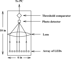
TWINKLE: Shamir’s factoring device

Adi Shamir has proposed the complete design of a (hardware) device, TWINKLE (The Weizmann INstitute Key Location Engine), that can perform the sieving stage of QSM a hundred to thousand times faster than software implementations in usual PCs available nowadays. This speed-up is obtained by using a high clock speed (10 GHz) and opto-electronic technology for detecting smooth integers. Each TWINKLE, if mass produced, has an estimated cost of US $5,000.

The working of TWINKLE is described in Figure 4.2. It uses an opaque cylinder of a height of about 10 inches and a diameter of about 6 inches. At the bottom of the cylinder is an array of LEDs,^[1] each LED representing a prime in the factor base. The i-th LED (corresponding to the i-th prime q_i) emits light of intensity proportional to log q_i. The device is clocked and the i-th LED emits light only during the clock cycles c for which q_i|T(c). The light emitted by all the active LEDs at a given clock cycle is focused by a lens and a photo-detector senses the total emitted light. If this total light exceeds a certain threshold, the corresponding clock cycle (that is, the time c) is reported to a PC attached to TWINKLE. The PC then analyses the particular T(c) for smoothness over {q₁, . . . , q_t} by trial division.

^[1] An LED (light emitting diode) is an electronic device that emits light, when current passes through it. A GaAs(Gallium arsenide)-based LED emits (infra-red) light of wavelength ~870 nano-meters. In the operational range of an LED, the intensity of emitted light is roughly proportional to the current passing through the LED.

Thus, TWINKLE implements incomplete sieving by opto-electronic means. The major difference between TWINKLE’s sieving and software sieving is that in the latter we used an array of times (the c values) and the iteration went over the set of small primes. In TWINKLE, we use an array of small primes and allow time to iterate over the different values of c in the sieving interval –M ≤ c ≤ M. An electronic circuit in TWINKLE computes for each LED the cycles c at which that LED is expected to emanate light. That is to say that the i-th LED emits light only in the clock cycles c congruent modulo q_i to any of the two solutions c₁ and of T(c) ≡ 0 (mod q_i). Shamir’s original design uses two LEDs for each prime q_i, one corresponding to c₁, the other to . In that case, each LED emits light at regularly spaced clock cycles and this simplifies the electronic circuitry (at the cost of having twice the number of LEDs).

Another difference of TWINKLE from software sieving is that here we add the log q_i values (to zero) instead of subtracting them from log |T(c)|. By Exercise 4.11, the values |T(c)| typically have variations by small constant factors. Taking logs reduces this variation further and, therefore, comparing the sum of the active log q_i values for a given c with a fixed predefined threshold (say log M H) independent of c is a neat way of bypassing the computation of all log |T(c)|, –M ≤ c ≤ M. (This strategy can also be used for software sieving.)

The reasons, why TWINKLE speeds up the sieving procedure over software implementations in conventional PCs, are the following:

Shamir [269] reports the full details of a VLSI^[2] design of TWINKLE.

^[2] very large-scale integration

*4.3.3. Factorization Using Elliptic Curves

H. W. Lenstra’s elliptic curve method (ECM) is another modern algorithm to solve the IFP and runs in expected time , where p is the smallest prime factor of n (the integer to be factored). Since , this running time is L[1] = L(n, 1/2, 1): that is, the same as the QSM. However, if p is small (that is, if p = O(n^α) for some α < 1/2), then the ECM is expected to outperform the QSM, since the working of the QSM is incapable of exploiting smaller values of p.

As before, let n be a composite natural number having no small prime divisors and let p be the smallest prime divisor of n. For denoting subexponential expressions in ln p, we use the symbol L_p[c] := L(p, 1/2, c), whereas the unsubscripted symbol L[c] stands for L(n, 1/2, c). We work with random elliptic curves

and consider the group of rational points on E modulo p. However, since p is not known a priori, we intend to work modulo n. The canonical surjection allows us to identify the -rational points on E as points on E over . We now define a bound and let B = {q₁, . . . , q_t} be all the primes smaller than or equal to M, so that by the prime number theorem (Theorem 2.20) #B ≈ M/ln . Of course, p is not known in advance, so that M and B are also not known. We will discuss about the choice of M and B later. For the time being, let us assume that we know some approximate value of p, so that M and B can be fixed, at least approximately, ate the beginning of the algorithm.

By Hasse’s theorem (Theorem 2.48, p 106), the cardinality satisfies , that is, ν = O(p). If we make the heuristic assumption that ν is a random integer on the order O(p), then Corollary 4.1 tells us that ν is B-smooth with probability . This assumption is certainly not rigorous, but accepting it gives us a way to analyse the running time of the algorithm.

If random curves are tried, then we expect to find one B-smooth value of ν. In this case, a non-trivial factor of n can be computed with high probability as follows. Define e_i := ⌊ln n/ln q_i⌋ for i = 1, . . . , t, and , where t is the number of primes in B. If ν is B-smooth, then ν|m and, therefore, for any point we have . Computation of mP involves computation of many sums P₁ + P₂ of points P₁ := (h₁, k₁) and P₂ := (h₂, k₂). At some point of time, we would certainly compute , that is, P₁ = –P₂, that is, h₁ ≡ h₂ (mod p) and k₁ ≡ –k₂ (mod p). Since p was unknown, we worked modulo n, that is, the values of h₁, h₂, k₁ and k₂ are known modulo n. Let d := gcd(h₁ – h₂, n). Then p|d and if d ≠ n (the case d = n has a very small probability!), we have the non-trivial factor d of n. The computation of the coordinates of P₁ + P₂ (assuming P₁ ≠ P₂) demands computing the inverse of h₁ – h₂ modulo n (Section 2.11.2). However, if d = gcd(h₁ – h₂, n) ≠ 1, then this inverse does not exist and so the computation of P₁ + P₂ fails, and we have a non-trivial factor of n. If ν is B-smooth, then the computation of mP is bound to fail. The basic steps of the ECM are then as shown in Algorithm 4.3.

Algorithm 4.3. Elliptic curve method (ECM)

Input: A composite integer (with no small prime factors). Output: A non-trivial divisor d of n. Steps: while (1) {    Select a random curve E : Y2 = X3 + aX + b modulo n.    Choose a point  in .    Try to compute mP.   /* where m is as defined in the text */    if (the computation of mP fails) {        /* We have found a divisor d > 1 of n */        if (d ≠ n) { Return d. }    } }

Before we derive the running time of the ECM, some comments are in order. A random curve E is chosen by selecting random integers a and b modulo n. It turns out that taking a as single-precision integers and b = 1 works quite well in practice. Indeed one can keep on trying the values a = 0, 1, 2, . . . successively. Note that the curve E is an elliptic curve, that is, non-singular, if and only if δ := gcd(n, 4a³ + 27b²) = 1. However, having δ > 1 is an extremely rare occurrence and one might skip the computation of δ before starting the trial with a curve. The choice b = 1 is attractive, because in that case we may take the point P = (0, 1). In Section 3.6, we have described a strategy to find a random point on an elliptic curve over a field K. This is based on the assumption that computing square roots in K is easy. The same method can be applied to curves over , but n being composite, it is difficult to compute square roots modulo n. So taking b to be 1 (or the square of a known integer) is indeed a pragmatic decision. After all, we do not need P to be a random point on E.

Recall that we have taken , where e_i = ⌊ln n/ln q_i⌋. If instead we take e_i := ⌊ln M/ln q_i⌋ (where M is the bound mentioned earlier), the computation of mP per trial reduces much, whereas the probability of a successful trial (that is, a failure of computing mP) does not decrease much. The integer m can be quite large. One, however, need not compute m explicitly, but proceed as follows: first take Q₀ := P and subsequently for each i = 1, . . . , t compute . One finally gets mP = Q_t.

Now comes the analysis of the running time of the ECM. We have fixed the parameter M to be , so that B contains small primes. The most expensive part of a trial with a random elliptic curve is the (attempted) computation of the point mP. This involves additions of points. Since an expected number of elliptic curves needs to be tried for finding a non-trivial factor of n, the algorithm performs an expected number of additions of points on curves modulo n. Since each such addition can be done in polynomial time, the announced running time follows.

Note that is the optimal running time of the ECM and can be shown to be achieved by taking . But, in practice, p is not known a priori. Various ad hoc ways may be adopted to get around with this difficulty. One possibility is to use the worst-case bound . For example, for factoring integers of the form n = pq, where p and q are primes of roughly the same size, this is a good approximation for p. Another strategy is to start with a small value of M and increase M gradually with the number of trials performed. For larger values of M, the probability of a successful trial increases implying that less number of elliptic curves needs to be tried, whereas the time per iteration (that is, for the computation of mP) increases. In other words, the total running time of the ECM is apparently not very sensitive to the choice of M.

A second stage can be used for each elliptic curve in order to increase the probability of a trial being successful. A strategy very similar to the second stage of the p – 1 method can be employed. The reader is urged to fill out the details. Employing the second stage leads to reasonable speed-up in practice, though it does not affect the asymptotic running time.

The ECM can be effectively parallelized, since different processors can carry out the trials, that is, computations of mP (together with the second stage) with different sets of (random) elliptic curves.

**4.3.4. The Number Field Sieve Method

The number field sieve method (NFSM) is till date the most successful of all integer factoring algorithms. Under certain heuristic assumptions it achieves a running time of the form L(n, 1/3, c), which is better than the L(n, 1/2, c′) algorithms described so far. The NFSM was first designed for integers of a special form. This variant of the NFSM is called the special NFS method (SNFSM) and was later modified to the general NFS method (GNFSM) that can handle arbitrary integers. The running time of the SNFSM has c = (32/9)^1/3 ≈ 1.526, whereas that for the GNFSM has c = (64/9)^1/3 ≈ 1.923. For the sake of simplicity, we describe only the SNFSM in this book (see Cohen [56] and Lenstra and Lenstra [165] for further details).

We choose an integer and a polynomial such that f(m) ≡ 0 (mod n). We assume that f is irreducible in ; otherwise a non-trivial factor of f yields a non-trivial factor of n. Consider the number field . Let d := deg f be the degree of the number field K. We use the complex embedding for some root of f. The special NFS method makes certain simplifying assumptions:

Consider the ring homomorphism

This is well-defined, since f(m) ≡ 0 (mod n). We choose small coprime (rational) integers a, b and note that Φ(a+bα) = a + bm (mod n). Let be a predetermined smoothness bound. Assume that for a given pair (a, b), both a + bm and a + bα are B-smooth. For the rational integer a + bm, this means

being the set of all rational primes ≤ B. On the other hand, smoothness of the algebraic integer a + bα means that the principal ideal is a product of prime ideals of prime norms ≤ B; that is, we have a factorization

where is the set of all prime ideals of of prime norms ≤ B. By assumption, each is a principal ideal. Let denote a set of generators, one for each ideal in . Further let denote a set of generators of the multiplicative group of units of . The smoothness of a + bα can, therefore, be rephrased as

Equation 4.4

Applying Φ then yields

This is a relation for the SNFSM. After relations are available, Gaussian elimination modulo 2 (as in the case of the QSM) is expected to give us a congruence of the form

x² ≡ y² (mod n),

and gcd(x – y, n) is possibly a non-trivial factor of n. This is the basic strategy of the SNFSM. We clarify some details now.

Selecting the polynomial f(X)

There is no clearly specified way to select the polynomial f for defining the number field . We require f to have small coefficients. Typically, m is much smaller than n and one writes the expansion of n in base m as n = b_tm^t + b_t–1m^t–1 + ··· + b₁m + b₀ with 0 ≤ b_i < m. Taking f(X) = b_tX^t + b_t–1X^t–1 + ··· + b₁X + b₀ is often suggested.

For integers n of certain special forms, we have natural choices for f. The seminal paper on the NFSM by Lenstra et al. [167] assumes that n = r^e – s for a small integer and a non-zero integer s with small absolute value. In this case, one first chooses a small extension degree and sets m := r^⌈e/d⌉ and f(X) := X^d – sr^{⌈e/d⌉d–e}. Typically, d = 5 works quite well in practice. Lenstra et al. report the implementation of the SNFSM for factoring n = 3²³⁹ – 1. The parameters chosen are d = 5, m = 3⁴⁸ and f(X) = X⁵ – 3. In this case, is monogenic and a PID.

Construction of

Take a small rational prime . From Section 2.13, it follows that if is the factorization of the canonical image of f(X) modulo p, then , i = 1, . . . , r, are all the primes lying over p. We have also seen that , , is prime if and only if d_i = 1, that is, for some . Thus, each root of in corresponds to a prime ideal of of prime norm p.

To sum up, a prime ideal in of prime norm is specified by a pair (p, c_p) of values (in ). We denote this ideal by . All ideals in can be precomputed by finding the roots of the defining polynomial f(X) modulo the small primes p ≤ B. One can use the root-finding algorithms of Exercise 3.29.

Construction of

Constructing a set of generators of ideals in is a costly operation. We have just seen that each prime ideal of corresponds to a pair (p, c_p) and is a principal ideal by assumption. A generator of such an ideal is an element of the form , , with N(g_p,cp) = ±p and (mod p). Algorithm 4.4 (quoted from Lenstra et al. [167]) computes the generators g_p,cp for all relevant pairs (p, c_p). The first for loop exhaustively searches over all small polynomials h(α) in order to locate for each (p, c_p) an element of norm kp with |k| as small as possible. If the smallest k (stored in a_p,cp) is ±1, is already a generator g_p,cp of , else some additional adjustments need to be performed.

Algorithm 4.4. Construction of generators of ideals for the SNFSM

Choose two suitable positive constants aB and CB (depending on B and K). Initialize an array ap,cp := aB indexed by the relevant pairs (p, cp). for each , , with , N(h) = kp, p ≤ B,       {0}, |k| < min(p, aB) {     Find cp such that .    /* Root finding */     if (|k| < |ap,cp|) {        /* Store the least k and the corresponding h found so far */        ap,cp := k, .     } } for each relevant pair (p, cp) {     if (ap,cp = ±1)    /* The more frequent case */     else {        Locate a  with N(g) = ap,cp.        .     } }

Construction of

Let K have the signature (r₁, r₂). Write ρ = r₁ + r₂ – 1. By Dirichlet’s unit theorem, the group of units of is generated by an appropriate root u₀ of unity and ρ multiplicatively independent^[3] elements u₁, . . . , u_ρ of infinite order. Each unit u of has norm N(u) = ±1. Thus, one may keep on generating elements , h_i small integers, of norm ±1, until ρ independent elements are found. Many elements of are available as a by-product during the construction of , which involves the computation of norms of many elements in . For a more general exposition on this topic, see Algorithm 6.5.9 of Cohen [56].

^[3] The elements u₁, . . . , u_ρ in a (multiplicatively written) group are called (multiplicatively) independent if , , is the group identity only for n₁ = ··· = n_ρ = 0.

Computing the factorization of a + bα

In order to compute the factorization of Equation (4.4), we first factor the integer N(a + bα) = b^df(–a/b). If is the prime factorization of 〈a + bα〉 with pairwise distinct prime ideals of , by the multiplicative property of norms we obtain .

Now, let p ≤ B be a small prime. If p  N(a + bα), it is clear that no prime ideal of of norm p (or a power of p) appears in the factorization of 〈a + bα〉. On the other hand, if p| N(a + bα), then for some . The assumption implies that the inertial degree of is 1: that is, , that is, , that is, there is a c_p with f(c_p) ≡ 0 (mod p) such that the prime ideal corresponds to the pair (p, c_p). In this case, we have a ≡ –c_pb (mod p). Assume that another prime ideal of norm p appears in the prime factorization of 〈a + bα〉. If corresponds to the pair p, , then . Since c_p and are distinct modulo p, it follows that p|gcd(a, b), a contradiction, since gcd(a, b) = 1. Thus, a unique ideal of norm p appears in the factorization of 〈a + bα〉. Moreover, the multiplicity of in the factorization of 〈a + bα〉 is the same as the multiplicity v_p(N(a + bα)).

Thus, one may attempt to factorize N(a + bα) using trial divisions by primes ≤ B. If the factorization is successful, that is, if N(a + bα) is B-smooth, then for each prime divisor p of N(a + bα) we find out the ideal and its multiplicity in the factorization of 〈a + bα〉 as explained above. Since we know a generator of each , we eventually compute a factorization , where u is a unit in . What remains is to factor u as a product of elements of . We don’t discuss this step here, but refer the reader to Lenstra et al. [167].

Sieving

In the QSM, we check the smoothness of a single integer T(c) per trial, whereas for the NFS method we do so for two integers, namely, a + bm and N(a + bα). However, both these integers are much smaller than T(c), and the probability that they are simultaneously smooth is larger than the probability that T(c) alone is smooth. This accounts for the better asymptotic performance of the NFS method compared to the QSM.

One has to check the smoothness of a + bm and N(a + bα) for each coprime a, b in a predetermined interval. This check can be carried out efficiently using sieves. We have to use two sieves, one for filtering out the non-smooth a + bm values and the other for filtering out the non-smooth a + bα values. We should have gcd(a, b) = 1, but computing gcd(a, b) for all values of a and b is rather costly. We may instead use a third sieve to throw away the values of a for a given b for which gcd(a, b) is divisible by primes ≤ B. This still leaves us with some pairs (a, b) for which gcd(a, b) > 1. But this is not a serious problem, since such values are small in number and can be later discarded from the list of pairs (a, b) selected by the smoothness test.

We fix b and allow a to vary in the interval –M ≤ a ≤ M for a predetermined bound M. We use an array indexed by a. Before the first sieve we initialize this array to . We may set for those values of a for which gcd(a, b) is known to be > 1 (where +∞ stands for a suitably large positive value). For each small prime p ≤ B and small exponent , we compute a′ := –mb (mod p^h) and subtract ln p from for each a, –M ≤ a ≤ M, with a ≡ a′ (mod p^h). Finally, for each value of a for which is not (close to) 0, that is, for which a + mb is not B-smooth, we set . For the other values of a, we set . One may use incomplete sieving (with a liberal selection criterion) during the first sieve.

The second sieve proceeds as follows. We continue to work with the value of b fixed before the first sieve and with the array available from the first sieve. For each prime ideal , we compute a″ := –bc_p (mod p) and subtract ln p from each location for which a ≡ a″ (mod p). For those a for which ln B for some real ξ ≥ 1, say ξ = 2, we try to factorize a + bα over and . If the attempt is successful, both a + bm and a + bα are smooth. This second sieve is an incomplete one and, therefore, we must use a liberal selection criterion.

The running time of the SNFSM

For deriving the running time of the SNFSM, take d ≤ (3 ln n/(2 ln ln n))^1/3, m = L(n, 2/3, (2/3)^1/3), B = L(n, 1/3, (2/3)^2/3) and M = L(n, 1/3, (2/3)^2/3). From the prime number theorem and from the fact that d is small, it follows that both and have the same asymptotic bound as B. Also meets this bound. We then have L(n, 1/3, (2/3)^2/3) unknown quantities on which we have to do Gaussian elimination.

The integers a + mb have absolute values ≤ L(n, 2/3, (2/3)^1/3). If the coefficients of f are small, then

|N(a + bα)| = |b^df(–a/b)| ≤ L(n, 1/3, d · (2/3)^2/3) = L(n, 2/3, (2/3)^1/3).

Under the heuristic assumption that a + mb and N(a + bα) behave as random integers of magnitude L(n, 2/3, (2/3)^1/3), the probability that both these are B-smooth turns out to be L(n, 1/3, –(2/3)^2/3), and so trying L(n, 1/3, 2(2/3)^2/3) pairs (a, b) is expected to give us L(n, 1/3, (2/3)^2/3) relations. The entire sieving process takes time L(n, 1/3, 2(2/3)^2/3), whereas solving a sparse system in L(n, 1/3, (2/3)^2/3) unknowns can be done essentially in the same time. Thus the running time of the SNFSM is L(n, 1/3, 2(2/3)^2/3) = L(n, 1/3, (32/9)^1/3).

Exercise Set 4.3

4.6	For , define the harmonic numbers . Show that for each we have ln(m + 1) ≤ Hm ≤ 1 + ln m. [H] Deduce that the sequence Hm, , is not convergent. (Note, however, that the sequence Hm – ln m, , converges to the constant γ = 0.57721566 . . . known as the Euler constant. It is not known whether γ is rational or not.)
4.7	Let k, c, c′, α be positive constants with α < 1. Prove the following assertions. . L(n, α, c)L(n, α, c′) is of the form L(n, α, c + c′). (ln n)kL(n, α, c) is again of the form L(n, α, c). L(n, α, c)nk is of the form nk+o(1).
4.8	Let us assume that an adversary C has computing power to carry out 1012 floating point operations (flops) per second. Let A be an algorithm that computes a certain function P(n) using T(n) flops for an input . We say that it is infeasible for C to compute P(n) using algorithm A, if it takes ≥ 100 years for the computation or, equivalently, if T(n) ≥ 3.1536 × 1021. Find, for the following expressions of T(n), the smallest values of n that make the computation of P(n) by Algorithm A infeasible: T(n) = (ln n)3, T(n) = (ln n)10, T(n) = n, , T(n) = n1/4, T(n) = L[2], T(n) = L[1], T(n) = L[0.5], T(n) = L(n, 1/3, 2) and T(n) = L(n, 1/3, 1). (Neglect the o(1) terms in the definitions of L( ) and L[ ].)
4.9	Let be an odd integer and let r be the total number of distinct (odd) prime divisors of n. Show that for each integer a the congruence x2 ≡ a2 (mod n) has ≤ 2r solutions for x modulo n. If gcd(a, n) = 1, show that this congruence has exactly 2r solutions. [H]
4.10	Show that the problems IFP and SQRTP are probabilistic polynomial-time equivalent. [H]
4.11	In this exercise, we use the notations introduced in connection with the Quadratic Sieve method for factoring integers (Section 4.3.2). We assume that M ≪ H, since , whereas M = L[1]. Show that J ≤ 2H – 1. Prove that the average of the integers |T(c)|, –M ≤ c ≤ M, is and that the maximum of the same integers is |T(M)| = J + 2MH + M2 ≈ J + 2MH. Prove that the average and the maximum of the integers |T(c)|, 0 ≤ c ≤ 2M, are respectively J + 2MH + M(4M + 1)/3 ≈ J + 2MH and |T(2M)| = J + 4MH + 4M2 ≈ J + 4MH. Conclude that it is better to choose the sieving interval as –M ≤ c ≤ M instead of as 0 ≤ c ≤ 2M.
4.12	Reyneri’s cubic sieve method (CSM) Suppose that we want to factor an odd integer n. Suppose also that we know a triple (x, y, z) of integers satisfying x3 ≡ y2z (mod n) with x3 ≠ y2z (as integers). We assume further that |x|, |y|, |z| are all O(pξ) for some ξ, 1/3 < ξ < 1/2. Show that for integers a, b, c with a + b + c = 0 one has (x + ay)(x + by)(x + cy) ≡ y2T(a, b, c) (mod n), where T(a, b, c) := z + (ab + ac + bc)x + (abc)y = –b(b + c)(x + cy) + (z – c2x). If x, y, z = O(pξ), then T(a, b, c) is O(pξ) for small values of a, b, c. Let . Choose a factor base comprising all primes q1, . . . , qt with t = L[α] together with the integers x + ay, –M ≤ a ≤ M, M = L[α]. The size of the factor base is then L[α]. If T(a, b, c) with –M ≤ a, b, c ≤ M and a + b + c = 0 is qt-smooth, we get a relation for the CSM. Show that trying out the L[2α] pairs (a, b, c) gives us a set of linear congruences of the desired size under the heuristic assumption that the T(a, b, c) values behave as random integers on the order of pξ. Propose a strategy how these linear congruences can be combined (by Gaussian elimination) to get a quadratic congruence of the form u2 ≡ v2 (mod n). Design a sieve for checking the smoothness of the expressions T(a, b, c). [H] Show that the running time of the CSM is . Since ξ < 1/2, the CSM is more efficient than the QSM. For ξ ≈ 1/3, the running time is . (Remark: It is not known how we can efficiently obtain a solution of x3 ≡ y2z (mod n) with x3 ≠ y2z and |x|, |y|, |z| = O(pξ), ξ being as small as possible. For some particular values of n, say, for n of the form x3 – z with small z, a solution is naturally available.)
4.13	Sieve of Eratosthenes Two hundred years before Christ, Eratosthenes proposed a sieve (Algorithm 4.5) for computing all primes between 1 and a positive integer n. Prove the correctness of this algorithm and compute its running time. [H] Algorithm 4.5. The sieve of Eratosthenes Initialize to zero an array A indexed 2, . . . , n. for     if (Ak = 0) { for l = 2, . . . , ⌊n/k⌋ { Alk := 1. } } } for k = 2, . . . , n { if (Ak = 0) { Print “k is a prime”. } }
4.14	This exercise proposes an adaptation of the sieve of Eratosthenes for computing a random prime of a given bit length l. In Section 3.4.2, we have described an algorithm for this computation, that generates random (odd) integers of bit length l and checks the primality of each such integer, until a (probable) prime is found. An alternative strategy is to generate a random l-bit odd integer n and check the integers n, n + 2, n + 4, . . . for primality. Use sieving to design an algorithm that generalizes this second strategy in the sense that it checks for primality only those integers n + r, r = 0, 1, 2, . . . , M, n a random l-bit integer, which are not divisible by the first t primes. In practice, the values 100 ≤ t ≤ 10,000 and M = 10l work quite well. For cryptographic sizes, sieving typically speeds up the generation of naive primes 10 to 100 times. Generalize the sieve of Part (a) for the computation of safe and strong primes.