
4.8. The Subset Sum Problem
In this section, we assume that ![]() be a knapsack set. For
be a knapsack set. For ![]() , we are required to find out
, we are required to find out ![]() such that
such that ![]() , provided that a solution exists. In general, finding such a solution for ∊1, . . . , ∊n is a very difficult problem.[6] However, if the weights satisfy some specific bounds, there exist polynomial-time algorithms for solving the SSP.
, provided that a solution exists. In general, finding such a solution for ∊1, . . . , ∊n is a very difficult problem.[6] However, if the weights satisfy some specific bounds, there exist polynomial-time algorithms for solving the SSP.
[6] In the language of complexity theory, the decision problem of determining whether a solution of the SSP exists is NP-complete.
Let us first define an important quantity associated with a knapsack set:
Definition 4.5.
|
The density of the knapsack set |
If d(A) > 1, then there are, in general, more than one solutions for the SSP (provided that there exists one solution). This makes the corresponding knapsack set A unsuitable for cryptographic purposes. So we consider low densities: that is, the case that d(A) ≤ 1.
There are certain algorithms that reduce in polynomial time the problem of finding a solution of the SSP to that of finding a shortest (non-zero) vector in a lattice. Assuming that such a vector is computable in polynomial time, Lagarias and Odlyzko’s reduction algorithm [157] solves the SSP in polynomial time with high probability, if d(A) ≤ 0.6463. An improved version of the algorithm adapts to densities d(A) ≤ 0.9408 (see Coster et al. [64] and Coster et al. [65]). The reduction algorithm is easy and will be described in Section 4.8.1. However, it is not known how to efficiently compute a shortest non-zero vector in a lattice. The Lenstra–Lenstra–Lovasz (L3) polynomial-time lattice basis reduction algorithm [166] provably finds out a non-zero vector whose length is at most the length of a shortest non-zero vector, multiplied by a power of 2. In practice, however, the L3 algorithm tends to compute a shortest vector quite often. Section 4.8.2 deals with the L3 lattice basis reduction algorithm.
Before providing a treatment on lattices, let us introduce a particular case of the SSP, which is easily (and uniquely) solvable.
Definition 4.6.
|
A knapsack set {a1, . . . , an} with a1 < ··· < an is said to be superincreasing, if |
Algorithm 4.10 solves the SSP for a superincreasing knapsack set in deterministic polynomial time. The proof for the correctness of this algorithm is easy and left to the reader.
Algorithm 4.10. Solving the superincreasing knapsack problem
4.8.1. The Low-Density Subset Sum Problem
We start by defining a lattice.
Definition 4.7.
|
Let n,
We say that v1, . . . , vd constitute a basis of L. |
In general, a lattice may have more than one basis. We are interested in bases consisting of short vectors, where the concept of shortness is with respect to the following definition.
Definition 4.8.
|
Let v := (v1, . . . , vn)t and w := (w1, . . . , wn)t be two n-dimensional vectors in 〈v, w〉 := v1w1 + ··· + vnwn, and the length of v is defined as
|
For the time being, let us assume the availability of a lattice oracle which, given a lattice, returns a shortest non-zero vector in the lattice. The possibilities for realizing such an oracle will be discussed in the next section.
Consider the subset sum problem with the knapsack set A := {a1, . . . , an} and let B be an upper bound on the weights (that is, each ai ≤ B). For ![]() , we are supposed to find out
, we are supposed to find out ![]() such that
such that ![]() . Let L be the n+1-dimensional lattice in
. Let L be the n+1-dimensional lattice in ![]() generated by the vectors
generated by the vectors
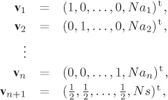
where N is an integer larger than ![]() . The vector
. The vector ![]() is in the lattice L, where
is in the lattice L, where ![]() . Involved calculations (carried out in Coster et al. [64, 65]) show that the probability P of the existence of a vector
. Involved calculations (carried out in Coster et al. [64, 65]) show that the probability P of the existence of a vector ![]() with ‖w‖ ≤ ‖v‖ satisfies
with ‖w‖ ≤ ‖v‖ satisfies ![]() , where c ≈ 1.0628. Now, if the density d(A) of A is less than 1/c ≈ 0.9408, then B = 2c′n for some c′ > c and, therefore, P → 0 as n → ∞. In other words, if d(A) < 0.9408, then, with a high probability, ±v are the shortest non-zero vectors of L. The lattice oracle then returns such a vector from which the solution ∊1, . . . , ∊n can be readily computed.
, where c ≈ 1.0628. Now, if the density d(A) of A is less than 1/c ≈ 0.9408, then B = 2c′n for some c′ > c and, therefore, P → 0 as n → ∞. In other words, if d(A) < 0.9408, then, with a high probability, ±v are the shortest non-zero vectors of L. The lattice oracle then returns such a vector from which the solution ∊1, . . . , ∊n can be readily computed.
4.8.2. The Lattice-Basis Reduction Algorithm
Let L be a lattice in ![]() specified by a basis of n linearly independent vectors v1, . . . , vn. We now construct a basis
specified by a basis of n linearly independent vectors v1, . . . , vn. We now construct a basis ![]() of
of ![]() such that
such that ![]() (that is,
(that is, ![]() and
and ![]() are orthogonal to each other) for all i, j, i ≠ j. Note that
are orthogonal to each other) for all i, j, i ≠ j. Note that ![]() need not be a basis for L. Algorithm 4.11 is known as the Gram–Schmidt orthogonalization procedure.
need not be a basis for L. Algorithm 4.11 is known as the Gram–Schmidt orthogonalization procedure.
Algorithm 4.11. Gram–Schmidt orthogonalization
|
Input: A basis v1, . . . , vn of Output: The Gram–Schmidt orthogonalization Steps:
|
One can easily verify that ![]() constitute an orthogonal basis of
constitute an orthogonal basis of ![]() . Using these notations, we introduce the following important concept:
. Using these notations, we introduce the following important concept:
Definition 4.9.
|
The basis v1, . . . , vn is called a reduced basis of L, if Equation 4.16
and Equation 4.17
|
A reduced basis v1, . . . , vn of L is termed so, because the vectors vi are somewhat short. More precisely, we have Theorem 4.5, the proof of which is not difficult, but is involved, and is omitted here.
Theorem 4.5.
|
Let v1, . . . , vn be a reduced basis of a lattice L, and
for all i = 1, . . . , m. In particular, for any non-zero vector w of L we have ‖ v1‖2 ≤ 2n–1‖w‖2. That is, for a reduced basis v1, . . . , vn of L the length of v1 is at most 2(n–1)/2 times that of the shortest non-zero vector in L. |
Given an arbitrary basis v1, . . . , vn of a lattice L, the L3 basis reduction algorithm computes a reduced basis of L. The algorithm starts by computing the Gram–Schmidt orthogonalization ![]() of v1, . . . , vn. The rational numbers μi,j are also available from this step. We also obtain as byproducts the numbers
of v1, . . . , vn. The rational numbers μi,j are also available from this step. We also obtain as byproducts the numbers ![]() for i = 1, . . . , n.
for i = 1, . . . , n.
Algorithm 4.12 enforces Condition (4.16) |μk,l| ≤ 1/2 for a given pair of indices k and l. The essential work done by this routine is subtracting a suitable multiple of vl from vk and updating the values μk,1, . . . , μk,l accordingly.
Algorithm 4.12. Subroutine for basis reduction
|
Input: Two indices k and l. Output: An update of the basis vectors to ensure |μk,l| ≤ 1/2. Steps:
vk := vk – rvl. for h = 1, . . . , l – 1 {μk,h := μk,h – rμl,h. } μk,l := μk,l – r. |
If Condition (4.17) is not satisfied by some k, that is, if ![]() , then vk and vk–1 are swapped. The necessary changes in the values Vk, Vk–1 and certain μi,j’s should also be incorporated. This is explained in Algorithm 4.13.
, then vk and vk–1 are swapped. The necessary changes in the values Vk, Vk–1 and certain μi,j’s should also be incorporated. This is explained in Algorithm 4.13.
Algorithm 4.13. Subroutine for basis reduction
|
Input: An index k. Output: An update of the basis vectors to ensure Steps: μ := μk,k–1. V := Vk + μ2Vk–1. |
The main basis reduction algorithm is described in Algorithm 4.14. It is not obvious that this algorithm should terminate at all. Consider the quantity D := d1 · · · dn–1, where di := | det(〈vk, vl〉)1≤k,l≤i| for each i = 1, . . . , n. At the beginning of the basis reduction procedure one has di ≤ Bi for all i = 1, . . . , n, where B := max(|vi|2 | 1 ≤ i ≤ n). It can be shown that an invocation of Algorithm 4.12 does not alter the value of D, whereas interchanging vi and vi–1 in Algorithm 4.13 decreases D by a factor < 3/4. It can also be shown that for any basis of L the value D is bounded from below by a constant which depends only on the lattice. Thus, Algorithm 4.14 stops after finitely many steps.
Algorithm 4.14. Basis reduction in a lattice
|
Input: A basis v1, . . . , vn of a lattice L. Output: v1, . . . , vn converted to a reduced basis. Steps: Compute the Gram–Schmidt orthogonalization of v1, . . . , vn (Algorithm 4.11). /* The initial values of μi,j and Vi are available at this point */ |
For a more complete treatment of the L3 basis reduction algorithm, we refer the reader to Lenstra et al. [166] (or Mignotte [203]). It is important to note here that the L3 basis reduction algorithm is at the heart of the Lenstra–Lenstra–Lovasz algorithm for factoring a polynomial in ![]() . This factoring algorithm indeed runs in time polynomially bounded by the degree of the polynomial to be factored and is one of the major breakthroughs in the history of symbolic computing.
. This factoring algorithm indeed runs in time polynomially bounded by the degree of the polynomial to be factored and is one of the major breakthroughs in the history of symbolic computing.