
84 5. THE PRESENT
Table 5.3: e three constituents of the universe, along with our degree of understanding of each
Component Percentage of the Universe Amount of our Knowledge
Normal matter 5% A lot
Dark matter 26% Very little
Dark energy 69% Almost nothing
5.4.5 THE DARK MATTER DENSITY (
c
)
ere is evidence, accumulated over many years, that much of the gravity in the universe—and
thus much of the mass—produces no light, nor is it otherwise affected by normal matter. We
call this unseen matter dark matter. We can detect dark matter even though it is invisible; it still
has gravity, and so it affects the motions of ordinary baryonic matter that we can see.
e most compelling idea currently is that dark matter is some type of hitherto undetected
subatomic particle that has properties quite unlike the familiar types that make up atoms. It is
proposed that these weakly-interacting massive particles (WIMPS) have mass—and thus gravity.
But they do not produce or otherwise interact with light. Nor are they affected by ordinary
matter, except through gravity.
e current estimates are that dark matter makes up about 26% of the universe—and so
there is roughly five times as much dark matter as ordinary (baryonic) matter.
5.4.6 THE DARK ENERGY DENSITY (
)
Beginning in the late 1990s, evidence accrued that suggests the expansion rate of the universe
is currently speeding up. is was both a surprising and transforming discovery; much obser-
vational data suddenly fit together better than ever before into one complete whole. But on the
other hand, the physical explanation for this accelerating expansion is unknown. e more-or-less
agreed upon name for this observed accelerating effect is dark energy.
Observations suggest that dark energy is the biggest component of the universe, accounting
for 69%, as opposed to 26% for dark matter and only 5% for normal matter. And so we are left
with the odd circumstance illustrated by Table 5.3. What seems to be most prominent in the
universe is what we understand least.
5.4.7 THE COSMIC MICROWAVE BACKGROUND TEMPERATURE (T)
e cosmic microwave background (CMB) is a dim glow of microwaves seen in every direction.
Its most compelling explanation is that it is radiation left over from when the universe was
extremely hot and dense. We will have much more to say about it, but it can be described very
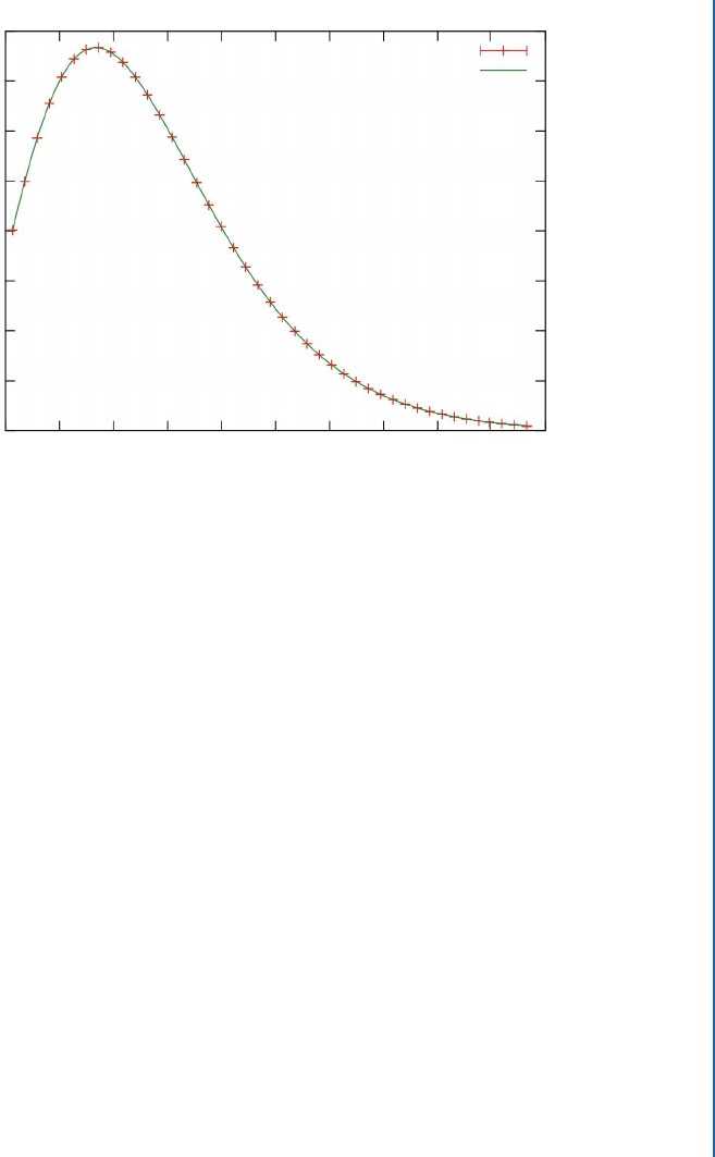
precisely by its temperature. Figure 5.3 shows the precisely measured energy distribution of the
5.4. COSMOLOGICAL PARAMETERS 85
400
350
200
250
200
150
100
50
0
2 4 6 8 10 12 14 16 18 20 22
COBE Data
Black Body Spectrum
Cosmic Microwave Background Spectrum (from COBE)
Frequency (1/cm)
Intensity (MJy/sr)
Figure 5.3: e observed spectrum of the cosmic microwave background together with a theo-
retical curve for a temperature of 2.73 K. e error bars for the observed data are too small to
show on the diagram. (Graphic by Quantum Doughnut, Public Domain.)
CMB, along with a theoretical curve with a temperature of 2.73 K, less than three degrees above
absolute zero.
5.4.8 THE CHEMICAL COMPOSITION OF THE UNIVERSE (XYZ)
e light we receive from stars, galaxies, and clouds of gas can tell us many things about the
matter from which it was emitted. In particular, an analysis of the spectrum of the light often
allows us to determine—sometimes to high precision—the chemical composition of the gases
that emitted the light. We explore how that works in more detail in Part IV of e Big Picture,
but let us here look at the results. What kinds of atoms are stars, galaxies, and clouds of gas and
dust typically made of?
e answer turns out to be the same over and over again, no matter where we look. Overall,
the universe seems to be made everywhere of very roughly these percentages of atoms (more
precise average values can be seen in Table 5.2):
• 3/4 Hydrogen,
• 1/4 Helium, and
• 0–2% Everything else put together.
86 5. THE PRESENT
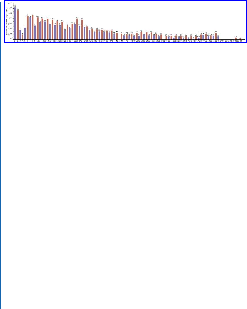
Figure 5.4: e relative abundances of the chemical elements in the solar system, portrayed on
a logarithmic scale. e horizontal axis is atomic number (number of protons in the atom).
(Graphic by Swift, CC0.)
is pattern repeats itself over and over. ere are variations; sometimes the helium abun-
dance is a little higher and the hydrogen abundance a little lower. And the small percentage of
“everything else put together” varies between nearly zero and about 2% or so. But even in this
case, the similarities are intriguing. For those other elements besides hydrogen and helium tend
to vary from place to place with nearly the same abundances relative to each other.
Since it is tiresome to keep repeating “everything else put together,” or “everything but
hydrogen and helium,” a word is needed. For historical reasons, astronomers use the rather
unfortunate term metals to refer to all of the elements, taken collectively, besides hydrogen and
helium. is would make a chemist cringe; the most common of the “metals” astronomers refer
to are carbon (C), nitrogen (N), and oxygen (O). ese three are about as non-metallic as an
element can be. To add insult to injury, we refer to an astronomical object’s percentage abundance
of metals with the totally-made-up-by-astronomers word metallicity.
ere are intriguing patterns in the abundances of “metals”:
• Roughly speaking, the more massive an atom is, the less abundant it is in the universe.
• Atoms with an odd number of protons are slightly less abundant than atoms with an even
number of protons.
We will have much to say about these facts later, in Section 9.11. But here we note that these
patterns hold for both relatively large and small overall abundances of the metals.
See Figure 5.4 for an illustration of the abundances of atoms in the solar system. is is
just a tiny dot in the universe, but most of the matter in the solar system is the Sun; the planets
add very little to the total. And so the relative abundances show in Figure 5.4 are very close to
those for the Sun itself. And the Sun is a rather typical star—albeit a star with comparatively high
metallicity. Note the overall pattern of decreasing abundance with number of protons, and the
zig-zag alternating pattern of high and low abundance from even-numbered to odd-numbered
elements.
Figure 5.4 shows the relative abundances on a logarithmic scale; looking at the numbers on
the vertical axis, we can see that carbon, for example, is thousands of times less abundant than
..................Content has been hidden....................
You can't read the all page of ebook, please click here login for view all page.