
Today, virtually all recorded signals are going to enter the ‘digital domain’ at some stage. It is beyond the scope of this book to explain the ‘mechanics’ of this process in any great depth, but a simplistic overview may help you understand where potential problems lurk.
‘The greatest invention since sliced bread’
A sound signal is a continuous and, for other than a steady tone, varying voltage (Figure 32.1). The first assumption in digitizing is that if you ‘look’ at that voltage once every ‘xth’ fraction of a second, and if ‘x’ is sufficiently small, replicating those values of voltage sequentially every ‘xth’ of a second thereafter will be indistinguishable, by ear, from the original continuous signal (Figure 32.2). Imagine a thinly sliced loaf of bread with every alternate slice removed. If the remaining slices of bread were to remain upright and in place, when viewed at an angle, the eye might be fooled into seeing a complete loaf.
The second assumption is that by ‘chopping’ the ‘columns’ of voltage up into a sufficient number of steps or levels and by assigning a numerical value of one ‘bit’ to each level, reproducing these values will again ‘fool’ the ear into hearing a continuous signal (Figure 32.3). Thus, the digitization process requires a sampling rate (every xth of a second) and a quantizing level to produce each ‘sliver’ or ‘column’ of signal. Imagine a child's building blocks. With the correct measurements you could easily replicate the height and outline shape of your own house, or car, or any other structure you care to name. But by now, you'll appreciate that you need lots of columns of blocks to faithfully reproduce these shapes. The same goes for digitizing, we first have to establish the parameters that will give us a sufficient number of ‘bits’ to faithfully replicate a signal without seeing or hearing the individual ‘blocks’.
So the quality of the reproduced signal relies on the number of samples per second and the number of quantizing (or digitizing) levels. The sampling rate must be more than twice the highest frequency to be reproduced, and the quantizing level must be sufficient to replicate a smooth sine wave (e.g. as produced by your tone oscillator). These factors determine the number of ‘bits’ the system must handle in real time.

Figure 32.1 The analogue sound signal
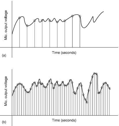
Figure 32.2 (a) The signal sampled at regular intervals, but in order to accurately represent the original, the sampling rate (every ‘xth’ of a second) must be at least twice the highest frequency that you wish to record (b)
Having done this, you're recording digital data – ‘ones’ and ‘noughts’. Every time the signal is reproduced, it's a ‘clone’ of the original, there is no perceptible loss in quality. However, to reduce the amount that has to be recorded, many systems compress the data. This is fine for one pass through a codec, which seeks to restore the signal to its original analogue values. But if the signal passes through a series of codecs, with different compression algorithms – for example, a signal path that consists of being recorded on tape or disc (first codec); transmitted via satellite (second), received and stored on a computer's hard disc (third); edited with software on a desk-top machine (fourth); and finally transmitted digitally from the server via a further compression system for both sound and pictures (fifth) – you can see how errors get the chance to multiply.
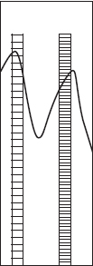
Figure 32.3 A closer look at a portion of the sampling. When quantizing each sample is assigned a number of digits depending on its voltage value at that point in time and the greater the number of steps/digits (bits) the more accurate the representation
Error handling
Nevertheless, anticipating problems in digital signals, extra information is added to assist the restoration of those portions of signal that have been lost. Error correction can reconstruct the digital signal exactly providing enough of the original remains intact (Figure 32.4). If errors continue to mount, error compensation interpolates (guesses) lost bits and reconstructs a ‘probability’ of the original signal. Too much ‘guessing’ leads to the picture displaying ‘blocky’ areas in frame (Figure 32.5) and some strange audio transitions or a ‘cracky’ or ‘gritty’ aspect to the sound.
The worst case scenario is when the errors exceed the capability of the system to interpolate, and the whole signal simply vanishes (Figure 32.6). Essentially, with a data stream of ‘ones and noughts’ you're dealing with on/off states, and a lack of sufficient information equates to off. This is both the strength and weakness of digital systems, their ability to handle errors and restore lost information is good, but when a problem overcomes this ability, the signal is lost in its entirety, and if the signal path is complex, it may take a long time to find and eliminate the fault.
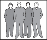
Figure 32.4 Error correction reproduces a perfect picture
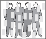
Figure 32.5 Error compensation, too much ‘guessing’ leads to ‘blocky’ pictures (and ‘gritty’ sound)

Figure 32.6 Too many errors overwhelm the correction/compensation system, result – no picture (or sound!)