
2.4. Natural convection in a nanofluid filled concentric annulus between an outer square cylinder and an inner circular cylinder
2.4.1. Problem definition and mathematical model
2.4.1.1. Problem statement
Fig. 2.19 shows the physical geometry considered in this study [13]. This geometry includes a concentric annulus between outer square and inner circular cylinders. The temperatures of inner and outer cylinders are considered Th and Tc, respectively (Th > Tc). In this figure γ is measured counterclockwise from the upward vertical plane through the center of outer cylinders and aspect ratio definition is λ = L/2r.

Figure 2.19 Geometry of the problem.
2.4.1.2. The lattice Boltzmann method
Two distribution functions, f and g, are used to simulate flow and temperature fields in thermal LBM. Macroscopic fluid quantities are calculated by simulating streaming and collision processes across a limited number of particles. Sample codes for LBM exist in the appendix. Fig. 2.20A shows the D2Q9 model which is used in this study. In this model values of  for |c0| = 0,
  for |c1–4| = 1, and
  for
for  must be assigned. Lattice Boltzmann equation (LBE) is solved to calculate density and temperature distribution functions. The general form of LBE with BGK approximation is introduced as follows:
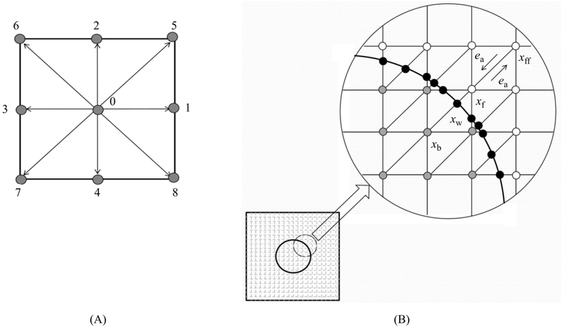
Figure 2.20 (A) Discrete velocity set of two-dimensional nine-velocity (D2Q9) model; (B) curved boundary and lattice nodes.
For the flow field:
 (2.77)
For the temperature field:
 (2.78)
where ci, ∆t, Fk denote the discrete lattice velocity in direction i, lattice time step, and external force in direction of lattice velocity, respectively. The lattice relaxation time for the flow and temperature fields are defined as  and
and  , respectively.
The equations for equilibrium distribution functions for flow and temperature are as follows:
 (2.79)
 (2.80)
where  and ρ are weighting factor and lattice fluid density, respectively. The buoyancy force in Eq. (2.77) is introduced as
Boussinesq approximation is considered for natural convection. Macroscopic variables can be calculated with following formula:
 (2.82)
2.4.1.2.1. Curved boundary treatment for velocity
Yan and Zu [14] proposed the model of applying curved boundaries for velocity and temperature fields. Fig. 2.20B shows an arbitrary curved wall. The fraction of the intersected link in the fluid region is defined as ∆ = |xf − xw|/|xf − xb|. Chapman–Enskog expansion for the postcollision distribution function on the right-hand side of Eq. (2.77) is used to estimate the postcollision distribution function  :
:
 (2.83)
where
 (2.84)
In the aforementioned formula,  ; uw, uf, and ubf are the velocity of solid wall, velocity of fluid, and an imaginary velocity for interpolations, respectively.
2.4.1.2.2. Curved boundary treatment for temperature
Temperature distribution function can be introduced as
 (2.86)
 (2.87)
where  is introduced as a function of Tb1 = [Tw+(∆−1)Tf]/∆ and Tb2 = [2Tw + (∆−1)Tff]/(1+∆)
 (2.88)
and  is introduced as a function of ub1 = [uw + (∆−1)uf]/∆ and ub2 = [2uw + (∆−1)uff]/(1+∆)
 (2.89)
2.5. The simulation of nanofluid in lattice Boltzmann model
Thermal characteristics should be changed to simulate nanofluid flow. Due to the extreme size and low concentration of the suspended nanoparticles, solid–liquid mixtures were considered as single-phase (homogenous) fluid. The base fluid is a water which contains different types of nanoparticles: Cu (copper), Al2O3 (alumina), Ag (silver), and TiO2 (titanium oxide). The effective density ρnf, the effective heat capacity (ρCp)nf, and thermal expansion (ρβ)nf of the nanofluid are introduced as
 (2.92)
where φ is the volume fraction of nanoparticles.
Brinkman model was used for simulation of viscosity of the nanofluid:
 (2.94)
The Maxwell–Garnetts (MG) model used to approximate the effective thermal conductivity of the nanofluid:
 (2.95)
Nusselt number is defined for comparison of total heat transfer rate. The local and average Nusselt numbers can be obtained as follows:
 (2.96)
The relaxation time for temperature (τC) is defined as τC = (3αnf + 0.5) where αnf = υ/Prnf and Prnf = μnf (Cp)nf/knf. Also, by fixing Rayleigh number, Prandtl number, and Mach number the viscosity is calculated from definition of:  where L is number of lattices in y-direction (parallel to gravitational acceleration). This Mach number should be less than 0.3 to insure an incompressible flow. Therefore, Mach number was fixed at Ma = 0.1 in the present study.
where L is number of lattices in y-direction (parallel to gravitational acceleration). This Mach number should be less than 0.3 to insure an incompressible flow. Therefore, Mach number was fixed at Ma = 0.1 in the present study.2.4.2. Effects of active parameters
One of the important key factors for heat transfer improvement is type of nanoparticles. Fig. 2.21 shows heat transfer augment because of adding different type of nanoparticles (Cu, Al2O3, Ag, and TiO2). This figure depicts that choosing copper as nanoparticles in most of the computations leads to the highest value of heat transfer enhancement. This study can be completed by considering the effects of nanoparticles volume fraction (φ = 0, 0.02, 0.04, and 0.06), Rayleigh number (Ra = 103, 104, 105, and 106) and aspect ratio (λ = 1.5–4.5) for Cu–water nanofluid on flow and heat transfer characteristics.
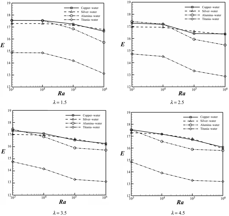
Figure 2.21 Ratio of enhancement of heat transfer due to addition of nanoparticles for different types of nanofluids when Pr = 6.8.
Fig. 2.22 shows the effect of adding nanoparticles on streamlines and isotherms for different values of aspect ratio when Ra = 106. This figure indicates that strength of flow increases by adding nanoparticle to the base fluid because of augment in the energy transport. Although thermal boundary layer thickness increases due to increase in nanoparticle volume fraction, Nusselt number has direct relationship with nanoparticle volume fraction.

Figure 2.22 Comparison of the isotherms (left) and streamlines (right) contours between nanofluid (φ = 0.06) (––) and pure fluid (φ = 0) (– –) for different values of λ at Ra = 106 and Pr = 6.8.
Isotherms and streamlines of nanofluid for different values of Rayleigh number when φ = 0.06, λ = 1.5 and 2.5 are depicted in Fig. 2.23. In this study streamlines and isotherms counters have symmetric shape about the vertical centerline. So for all cases just half of geometry is depicted. For λ = 2.5, streamline has two overall rotating symmetric eddies with two inner vortices at low Rayleigh number in which conduction heat transfer is more dominant. By increasing Rayleigh number up to 104, samples of isotherms and streamlines are not changed notably.

Figure 2.23 Effects of Rayleigh numbers (Ra) and aspect ratio (λ) on isotherms (left) and streamlines (right) contours for Cu–water case (φ = 0.06).
At Ra = 105, convective heat transfer becomes more considerable. A thermal plume appears over the circular cylinder. The core of eddies are placed in the upper half of enclosure because of domination of flow in this region. At Ra = 106, the thermal plume becomes stronger and thus thermal boundary layer thickness becomes thinner. For higher value of inner cylinder radius (λ = 1.5) the shapes of streamlines and isotherms are almost similar to those at λ = 2.5 when Ra = 103 and 104. As Rayleigh number increases up to Ra = 106, an interesting phenomenon is observed. The thermal plume squeezed the isotherms on the top of the enclosure. So, the primary plume dived into three plumes. It can be found that |ψmax| is higher at λ = 2.5 than at λ = 1.5 except for Ra = 106 because of more accessible space for flow circulation.
Fig. 2.24 illustrates flow and temperature distribution for λ = 3.5 and 4.5 at different values of Rayleigh number. At Ra = 103 two cells exist in streamlines and increasing Rayleigh number causes two cells to merge into one cell. As Rayleigh number increases up to Ra = 106 the center core of this single cell divides into two small cells. Also this figure shows that |ψmax| is higher for smaller aspect ratio except for Ra = 106 which is similar to the trend of |ψmax| at Fig. 2.23.
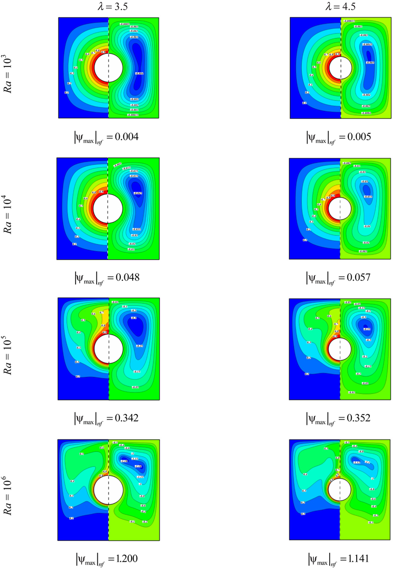
Figure 2.24 Effects of Rayleigh numbers (Ra) and aspect ratio (λ) and nanoparticle volume fraction (φ) on isotherms (left) and streamlines (right) contours for Cu–water case (φ = 0.06).
Figs. 2.25 and 2.26 display the distribution of the local Nusselt numbers only over the left half of the enclosure and inner cylinder. For all cases increasing nanoparticles volume fraction causes Nusselt number to increase. Also it can be found that the local Nusselt number profiles become smoother as the aspect ratio increases. As heat conduction is dominant mode of heat transfer in low Rayleigh numbers the local Nusselt number profiles have symmetric shape with respect to the horizontal centerline. Due to presence of three plumes at the region of the top wall of the enclosure, local Nusselt number profiles are more complex for the case of λ = 1.5, Ra = 105 and 106.
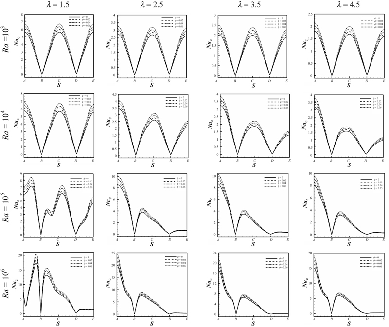
Figure 2.25 Effects of Rayleigh numbers (Ra) and aspect ratio (λ) and nanoparticles volume fraction (φ) on local Nusselt number along the walls of the enclosure (Nuc) for Cu–water case.
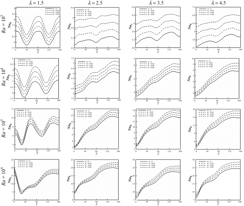
Figure 2.26 Effects of Rayleigh numbers (Ra), aspect ratio (λ) and nanoparticles volume fraction (φ) on local Nusselt number along the surface of the inner cylinder (Nuh) for Cu–water case.
The average Nusselt number over the surface of the enclosure  and over the inner cylinder
  as a function of aspect ratio (λ) for different Rayleigh numbers are shown in Fig. 2.27. The average Nusselt number on the both inner and outer cylinders has direct relationship with Rayleigh number and nanoparticle volume fraction. As aspect ratio decreases, Nusselt number increases due to reduction of the gap between cold and hot surfaces. Also it can be seen different behavior for
  when aspect ratio increases. At Ra = 103 and 104 the minimum value of is obtained at λ = 2.5 while has an increasing trend with respect to the aspect ratio for Ra = 105 and 106.
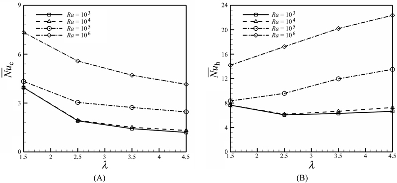
Figure 2.27 Effects of Ra and λ on (A)  ; (B)
; (B)  for Cu–water case when φ = 0.06.
Fig. 2.28 depicts the effects of aspect ratio and Rayleigh number on the heat transfer augment ratio due to addition of nanoparticles. The rate of heat transfer increases by adding nanoparticles; however, the rate of enhancement is greater for the enclosure with low Rayleigh number in which conduction heat transfer is more dominant. When Ra = 103 and 104, enhancement decreases with increase of aspect ratio whereas for other Rayleigh numbers λ = 2.5 roles as a critical aspect ratio. Moreover, the maximum value of E is related to λ = 2.5 at Ra = 106 whereas for other Rayleigh numbers it is obtained at λ = 1.5. This observation is related to this fact that conduction heat transfer is prominent in lower Rayleigh numbers. Hence in  and
and  , the maximum enhancement occurred for λ = 1.5 (when the distance between the hot inner and cold outer walls is minimum). At Ra = 106 convective heat transfer becomes more important. On the other hand, at λ = 1.5 the distance between hot and cold walls is more than that of λ = 2.5. Hence the fluid could easily circulate between the two cylinders and this phenomenon leads to the greater enhancement at λ = 1.5.

Figure 2.28 Effects of Ra and λ on E for Cu–water case.
2.5. Natural convection in a nanofluid filled concentric annulus with inner elliptic cylinder using LBM
2.5.1. Problem definition
The physical model used in this work is shown in Fig. 2.29 [15]. The model consists of a concentric annulus between a cold outer square cylinder with temperature Tc and a heated inner horizontal elliptic cylinder with temperature Th (Th>Tc). Setting a as the major axis and b as the minor axis of elliptic cylinder, the eccentricity (ɛ) for the inner cylinder is defined as
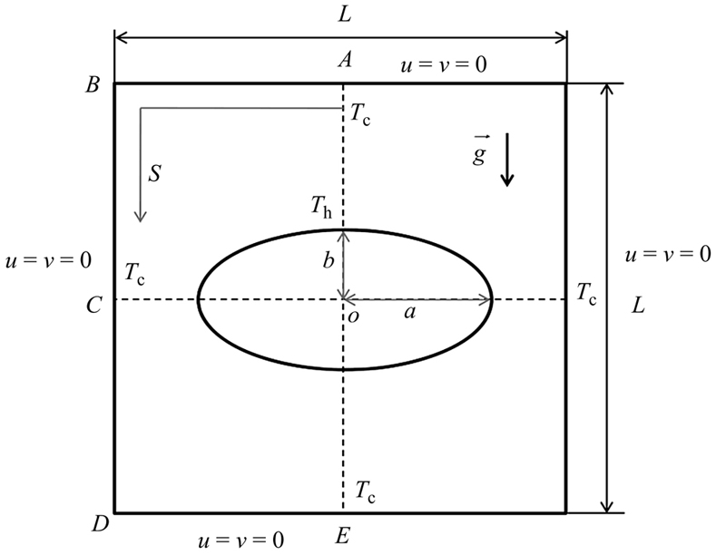
Figure 2.29 Geometry of the problem.
In this section, for the inner ellipse, the major axis is a = 0.4 and the eccentricity varies from 0.65 to 0.95.
2.5.2. Effects of active parameters
Natural convection in a concentric annulus between a cold outer square cylinder and a heated inner elliptic filled with nanofluid is investigated numerically using the LBM. The algorithm of this method is shown in Fig. 2.30. The fluid in the enclosure is Cu–water nanofluid. Calculations are made for different values of volume fraction of nanoparticle (φ = 0,0.02, 0.04, and 0.06), Rayleigh number (Ra = 103, 104, 105, and 106), and eccentricity (ɛ = 0.65, 0.8, and 0.95) when Prandtl number is fixed (Pr = 6.8) and major axis is a = 0.4.

Figure 2.30 Algorithm flowchart of lattice Boltzmann method.
Effects of Cu nanoparticles on the streamlines and isotherms are shown in Fig. 2.31. As seen the flow intensity increases with increase of nanoparticles volume fraction which enhances the energy transport within the fluid. Hence, the absolute values of stream function which represents the strength of flow increase with increasing the volume fraction of nanofluid. The sensitivity of thermal boundary layer thickness to volume fraction of nanoparticles is related to the increased thermal conductivity of the nanofluid. In fact, higher values of thermal conductivity are accompanied by higher values of thermal diffusivity. The high value of thermal diffusivity leads to increase in thermal boundary layer thickness. However, the Nusselt number is a multiplication of temperature gradient and the thermal conductivity ratio (conductivity of the nanofluid to the conductivity of the base fluid). As the reduction in temperature gradient due to the presence of nanoparticles is much smaller than the thermal conductivity ratio, an enhancement in Nusselt takes place by increasing the volume fraction of nanoparticles.
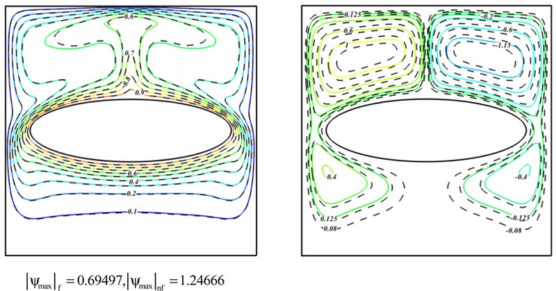
Figure 2.31 Comparison of the isotherms (left) and streamlines (right) contours between nanofluid (φ = 0.06) (––) and pure fluid (φ = 0) (– –) for Ra = 106 and φ = 0.06.
Effects of Ra and ɛ on isotherms (up) and streamlines (down) contours for Cu–water case (φ = 0.06) are shown in Fig. 2.32. As seen the absolute value of maximum stream function increases with increase of Rayleigh number and the eccentricity. It can be observed that the flow and temperature counters are generally symmetrical about the vertical centerline of the inner circular cylinder. At Ra = 103, the heat transfer in the enclosure is mainly dominated by the conduction mode and the flow circulation shows two overall rotating symmetric eddies with two inner vortices in each half of the enclosure. At Ra = 104, the patterns of isotherms and streamlines are about the same as those for Ra = 103. As the Rayleigh number increases up to 105, the role of convection in heat transfer becomes more significant and consequently the thermal boundary layer on the bottom surface of the inner cylinder becomes thinner. Also, a plume starts to appear on the top of the inner cylinder. In consequence, the dominant flow is in the upper half of the enclosure, and correspondingly the core of the recalculating eddies is located only in the upper half. At Ra = 106, a strong plume derives that the flow strongly impinges on the top of the enclosure. So thermal boundary layer thickness decreases in this region. For ɛ = 6.5 and low Rayleigh numbers Ra = 103 and 104 the isotherms and streamlines behave similar to those other values of ɛ. As the Rayleigh number increases up to Ra = 105 and 106, isotherms at the upper half of the enclosure are slightly squeezed and the temperature value at the vertical centerline is lower than that at the same height close to the vertical centerline. Thus the primary plume is divided into three plumes. Two upwelling plumes appear on the top of the inner cylinder. A third plume appears above the top of the inner circular cylinder with reverse direction owing to the two secondary vortices newly generated at this region.
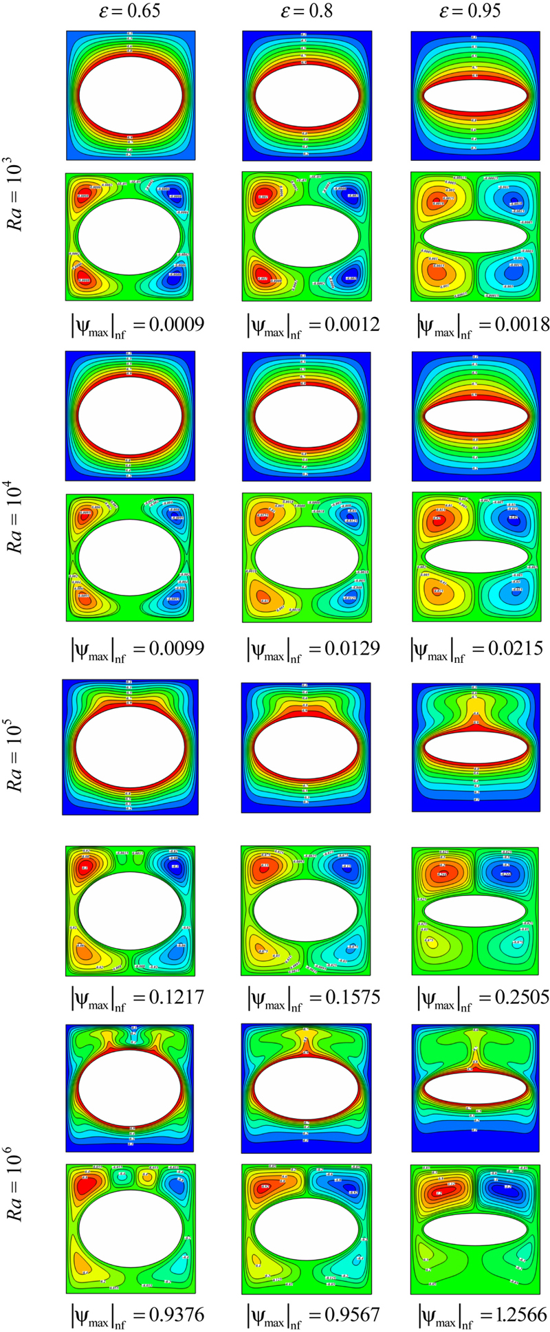
Figure 2.32 Effects of Ra and ɛ on isotherms (up) and streamlines (down) contours for Cu–water case (φ = 0.06).
Fig. 2.33 shows the effects of Ra, ɛ, and φ on the local Nusselt number along the surface of the outer cylinder (Nuloc). For all cases as nanoparticles volume fraction increases the value of local Nusselt number enhances. At Ra = 103, the isotherms show almost a symmetric shape with respect to the horizontal centerline because the dominant heat transfer mechanism is conduction and as a result the distribution of the local Nusselt numbers along the surface of the cold surface of the enclosure shows the symmetric shape. When we move from point A to B along the top wall of the enclosure, the local Nusselt number decreases and reaches a local minimum value close to zero at point B. When we move from point B to C along the right wall of the enclosure, the local Nusselt number increases, reaches a local maximum value, and decreases again until it has a local minimum value at point D. When we move further from point D to E, the local Nusselt number increases slightly again. The observed changes are most likely due to change in thermal boundary layer thickness. The local minimum and maximum values of local Nusselt number occur at the same point of Ra = 103 when Rayleigh number increases up to 104 but the local Nusselt profiles are not symmetric anymore. Because of generation of thermal plumes due to domination of convective heat transfer mechanism at high Rayleigh numbers, local Nusselt number profiles have more extremum. It is interesting to notice that local Nusselt number profile is more complex when Ra = 106 and ɛ = 6.5. This observation is due to the presence of three plumes at the vicinity of the top wall of the enclosure. By squeezing isotherms at the upper half of the enclosure, the primary plume is divided into three plumes. So, Nuloc have one maximum and one minimum point between A and B. Also in this case, there is one minimum point between B and D which is due to domination of conduction mechanism in this region.
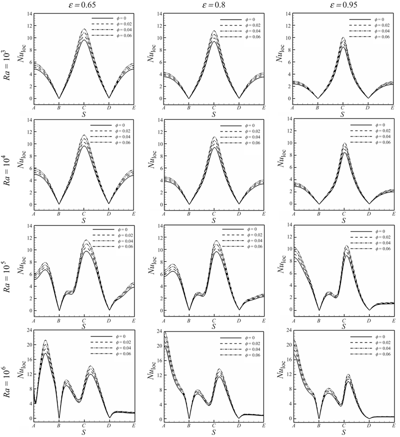
Figure 2.33 Effects of Ra, ɛ, and φ on local Nusselt number along the surface of the outer cylinder (Nuloc) for Cu–water case.
Fig. 2.34 shows effects of Ra and ɛ on average Nusselt number along the walls of the enclosure. Average Nusselt number has direct relationship with Rayleigh number and nanoparticles volume fraction but it has reverse relationship with the eccentricity. Effects of Ra and ɛ on ratio of enhancement of heat transfer due to addition of nanoparticles for Cu–water case are shown in Fig. 2.35. When ɛ = 0.65 and ɛ = 0.8, the effect of nanoparticles is more pronounced at low Rayleigh number than at high Rayleigh number domination of conduction heat transfer mechanism, whereas for ɛ = 0.95 enhancement of heat transfer decreases with increase of Rayleigh number when Ra ≤ 105 but it decreases when Ra > 105. When Ra = 103, 104, and 106 increase in the eccentricity leads to increase in En but for Ra = 105 opposite trend is observed.

Figure 2.34 Effects of Ra and ɛ on average Nusselt number along the walls of the enclosure (Nuave).

Figure 2.35 Effects of Ra and ɛ on ratio of enhancement of heat transfer due to addition of nanoparticles for Cu–water case.
2.6. Natural convection in a nanofluid filled square cavity with curve boundaries
2.6.1. Problem definition
The schematic diagram of square cavity with curve boundaries used in the present LBM program is shown in Fig. 2.36 [16]. The left and right walls are maintained at constant temperatures Th and Tc, respectively, while the two other walls are thermally insulated. Also γ is introduced as inclination angle. Furthermore,  and L are radius of curve boundary and length of adiabatic wall, respectively. We assume that R/L = 0.5.
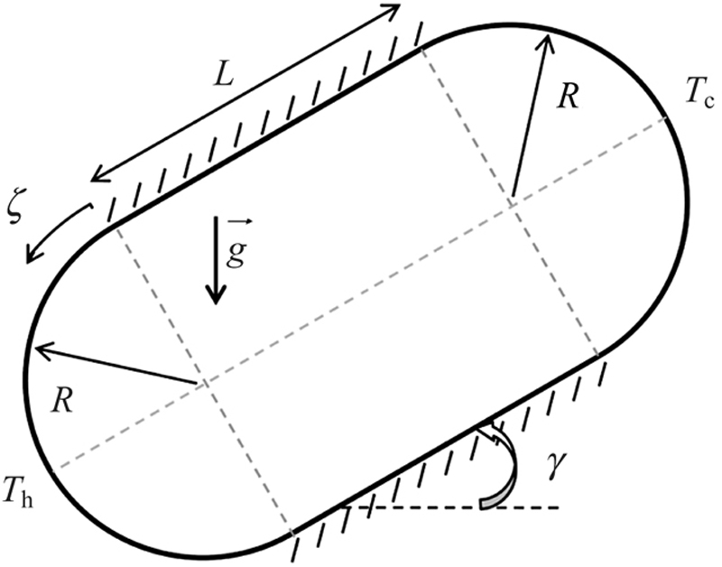
Figure 2.36 Geometry of the problem.
2.6.2. Effects of active parameters
Natural convection of Cu–water nanofluid in an inclined cavity with curve boundaries is investigated numerically using LBM. Calculations are made for various values of volume fraction of nanoparticle (φ = 0,0.02, 0.04, and 0.06), Rayleigh number (Ra = 103, 104, and 105), and inclination angle (γ = −60°, −30°, 0°, 30° to 60°) when Prandtl number is fixed (Pr = 6.8) and aspect ratios (R/L = 0.5).
Comparison of the isotherms (up) and streamlines (down) contours for different values of Rayleigh numbers and inclination angles is shown in Fig. 2.37. The calculated maximum values of absolute stream function are also given with each graph for reference. Here, as Rayleigh number increases |ψmax| increases. It can be seen that the change of inclination angle has a significant impact on the thermal and hydrodynamic flow field. In case, by increasing the Rayleigh number, streamlines start to penetrate toward the cavity center. When γ = 0°, at Ra = 103 streamlines have a single vortex whose center is located at the center of the system. At this Rayleigh number the conduction heat transfer mechanism is more pronounced and the isotherms are parallel to each other and also take the enclosure shape. As the Rayleigh number increases (Ra = 104), the central streamline is distorted into an elliptic shape due to higher flow velocity. At Ra = 105, the central streamline is elongated and two secondary vortices appear inside it. For case, γ = 0° when the hot surface is left, the isotherms are very dense near the bottom of the hot wall and the top of the cold wall and temperature gradient near the walls is very large, especially in higher Rayleigh numbers. According to streamlines in Fig. 2.37, the double vortex may occur when the hot wall is up. This fact is due to the existence of gravitational force which prevents fluid to flow from cold wall to the hot one. Also isotherms are more dense at the middle of enclosure. When the hot wall is located at the bottom, a single vortex is observed in the cavity.
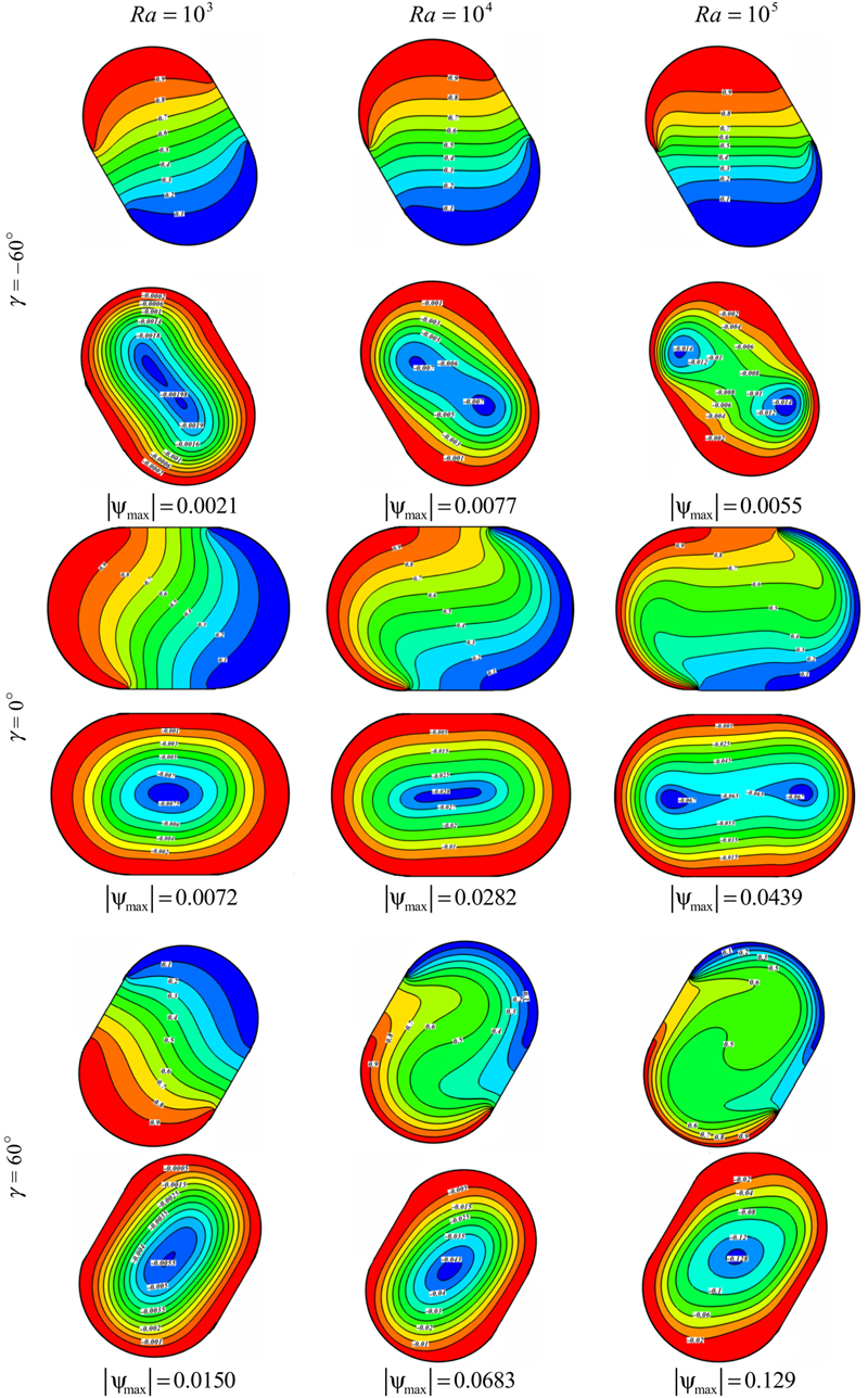
Figure 2.37 Comparison of the isotherms (up) and streamlines (down) contours for different values of Rayleigh numbers and inclination angles at φ = 0.06.
The variation of local Nusselt number along the hot surface at different inclination of cavity for three Rayleigh numbers is depicted in Fig. 2.38. It displays the influence of the Rayleigh number and the inclination angles on the local Nusselt number along the heated surface (Nuloc). As illustrated in Fig. 2.38, for low value of Rayleigh, local Nusselt number is approximately independent of inclination angle. The Nuloc increases with growth of Rayleigh number which is due to increase in convective heat transfer. It is observed that the local Nusselt number increases slightly with increase of inclination angle. For lower Rayleigh numbers, the trend of local Nusselt number variation is the same. In fact at low Rayleigh numbers, it is independent of the inclination angle variation. In addition, the most increasing rate of local Nusselt number occurs when ζ increases from 145° to 180°.
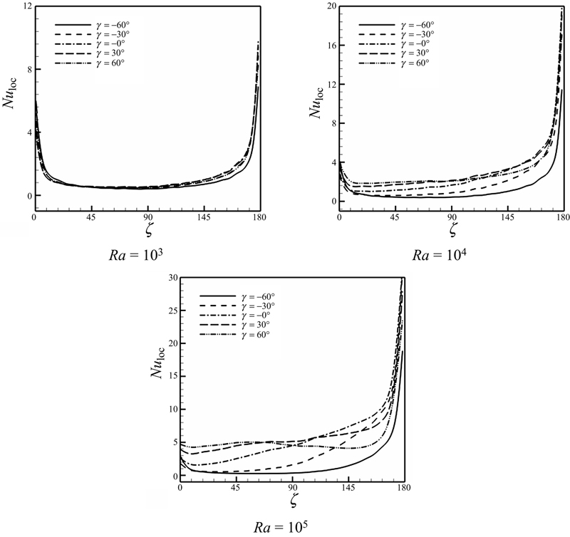
Figure 2.38 Effects of the Rayleigh number and inclination angle on local Nusselt number when φ = 0.06.
Effects of the volume fraction of nanoparticles, Rayleigh number, and inclination angle on average Nusselt number are shown in Fig. 2.39. The sensitivity of thermal boundary layer thickness to volume fraction of nanoparticles is related to the increased thermal conductivity of the nanofluid. In fact, higher values of thermal conductivity are accompanied by higher values of thermal diffusivity. The high value of thermal diffusivity causes a drop in the temperature gradients and accordingly increases the thermal boundary layer thickness. This increase in thermal boundary layer thickness reduces the Nusselt number; however, Nusselt number is a multiplication of temperature gradient and the thermal conductivity ratio (conductivity of the nanofluid to the conductivity of the base fluid). As the reduction in temperature gradient due to the presence of nanoparticles is much smaller than the thermal conductivity ratio, an enhancement in Nusselt number takes place by increasing the volume fraction of nanoparticles. As seen in Fig. 2.39, increasing Rayleigh number leads to increase in Nusselt number. Also it can be found that maximum value of Nusselt number occurs at γ = 0° for Ra = 103 but for other values of Rayleigh number maximum values of Nusselt number are obtained at γ = 30°. For all values of Rayleigh number minimum value of Nusselt number is obtained at γ = −60°.

Figure 2.39 Effects of the volume fraction of nanoparticles, Rayleigh number, and inclination angle on average Nusselt number when Pr = 6.8.
Heat transfer enhancement due to addition of nanoparticles for different values of Rayleigh number and inclination angle is shown in Fig. 2.40. For γ > 0°, the effect of nanoparticles is more pronounced at low Rayleigh number than at high Rayleigh number because of greater amount of rate of enhancement and increasing Rayleigh number leads to decrease in enhancement of heat transfer. For γ < 0° maximum values of enhancement occur at Ra = 105. Also it can be seen that at Ra = 103, enhancement profile has one maximum and one minimum point while for other values of Rayleigh number enhancement decreases with increase of γ.

Figure 2.40 Effects of the Rayleigh number and inclination angle on enhancement heat transfer.
2.7. Nanofluid heat transfer enhancement and entropy generation
2.7.1. Problem definition and governing equations
2.7.1.1. Problem definition
The physical geometry of the problem and coordinate system with related parameters are shown in Fig. 2.41 [17]. A rectangular body with height t and width H/2 is placed in the center of the square enclosure (of dimensions H by H), and is assumed to be isothermal at comparatively higher temperature as compared with the two vertical isothermal walls. The top and bottom walls are insulated.

Figure 2.41 Geometry of the problem.
2.7.1.2. The lattice Boltzmann method
The thermal LB model utilizes two distribution functions, f and g, for the flow and temperature fields, respectively. Thermal LBM employs modeling of movement of fluid particles to capture macroscopic fluid quantities, such as velocity, pressure, and temperature. In this approach, the fluid domain is discretized to uniform Cartesian cells. The probability of finding particles within certain range of velocities at a certain range of locations replaces tagging each particle as in the computationally intensive molecular dynamics simulation approach. In LBM, each cell holds a fixed number of distribution functions, which represent the number of fluid particles moving in these discrete directions. The D2Q9 model has been implemented and values of for |c0| = 0 (for the static particle), for |c1–4| = 1 and for are assigned in this model. The density and distribution functions, that is, f and g, are calculated by solving the LBE, which is a special discretization of the kinetic Boltzmann equation. After introducing the BGK approximation, the general form of LBE with external force is
For the flow field:
 (2.98)
For the temperature field:
(2.99)Here ∆t denotes lattice time step, ci is the discrete lattice velocity in direction i, Fk is the external force in direction of lattice velocity, τv and τC denote the lattice relaxation times for the flow and temperature fields. The kinetic viscosity υ and the thermal diffusivity α are defined in terms of their respective relaxation times, that is,  and
and  , respectively. Note that the limitation 0.5 < τ should be satisfied for both relaxation times to ensure that viscosity and thermal diffusivity are positive. Furthermore, the local equilibrium distribution function determines the type of problem being simulated. It also models the equilibrium distribution functions, which are calculated with Eqs. (2.100) and (2.101) for flow and temperature fields, respectively:
(2.100)
 (2.101)
where  is a weighting factor and ρ is the lattice fluid density.
To incorporate buoyancy force in the model, the force term in Eq. (2.98) has to be evaluated in the vertical direction (y):
where gy and β are gravitational acceleration and thermal expansion coefficients. For natural convection, the Boussinesq approximation is applied. To ensure that the thermal LBM code works in the near-incompressible regime, the characteristic velocity of the flow for the natural convection regime  must be small compared with the fluid speed of sound. In the present study, the characteristic velocity is adopted as 0.1 that of sonic speed. Finally, the macroscopic variables are computed with the following formulae:
 (2.103)
2.7.1.2.1. Boundary conditions
Bounce-back boundary conditions were applied on all solid boundaries, which indicate that incoming boundary populations are equal to outgoing populations after the collision. Bounce back type boundary conditions are proven to provide more accurate numerical approximations for LBM simulations. For instance, for the east boundary, the following conditions are imposed:
where n is the node on the lattice.
A bounce-back boundary condition (adiabatic) is used on the north and south of the boundaries. For instance at the north boundary, the following conditions are imposed:
Temperatures at the rectangular body and active side walls are known. For instance at the west boundary of rectangular body Th = 1, as we are using D2Q9, the unknowns are g3, g6, and g7 which are evaluated as
 (2.106)
2.7.1.2.2. Second law analysis
According to Bejan [18], one can find the volumetric entropy generation rate as
where HTI is the irreversibility due to heat transfer in the direction of finite temperature gradients and FFI is the contribution of fluid friction irreversibility to the total generated entropy.
In terms of the primitive variables, HTI and FFI become
 (2.108)
One can also define the Bejan number, Be, as
 (2.109)
Note that a Be value more/less than 0.5 shows that the contribution of HTI to the total entropy generation is higher/lower than that of FFI. The limiting value of Be = 1 shows that the only active entropy generation mechanism is HTI while Be = 0 represents no HTI contribution.
The dimensionless form of entropy generation rate, Ns, is defined as
 (2.110)
one finds that
 (2.111)
where the dimensionless temperature difference is defined as
 (2.112)
The dimensionless viscous dissipation function, addressed in Eq. (2.111), takes the following form:
 (2.113)
One easily verifies that, as both Ω and θ can put on values smaller than unity, one cannot neglect any of them in favor of the other as noted by Hooman and Ejlali [19] for a forced convection problem. Keep in mind that Ω can be O(1) for special cases. Hence, one should be very careful when one simply neglects either Ω−1 or θ in the denominator of Eq. (2.111). Here, Ge is the Gebhart number which is defined as
 (2.114)
and throughout this work Ge = 10−5 to be a real choice for most of engineering applications. In the light of Nield [20] one knows that the proper dimensionless number to show the effects of viscous dissipation in a free convection problem in a cavity, filled with or without a porous insert, is the Gebhart number which, interestingly, does not contain viscosity; see also Hooman et al. [21]. Unlike the previous findings of Dagtekin et al. [22], proper scaling shows that with a fixed Ge value FFI decreases with Ra. Interestingly, both HTI and Ns increase with Ra and this will be elaborated on in the forthcoming discussion. It should also be noted that there are certain cases where viscous dissipation effects are not important in the thermal energy equation but can be significant when it comes to study second law aspects of a convection problem as outlined by Bejan [18]. The local and average values of Be are found to convey little information as they are very close to unity; hence, we did not present any graph or contour for Be. Average Ns is denoted by [Ns], where the angle brackets show an average taken over the area, as
 (2.115)
Selecting the fluid, trapped between the heated plate and the cavity, as the thermodynamic system, one observes that the amount of heat entered through the heated plate is equal to the one transferred to the surroundings via the isothermal walls. Moreover, one notes that the total volumetric entropy generation rate is obtainable as
 (2.116)
where, in terms of Nu, it reads
 (2.117)
Applying perturbation techniques for small values of Ω, say Ω<<1, one has
 (2.118)
The dimensionless entropy generation number can be obtained as
 (2.119)
The average Nusselt numbers are defined as follows:
 (2.120)
2.7.2. Effects of active parameters
In this study natural convection in a square enclosures using nanofluid is investigated numerically using the LBM scheme. A rectangular heated body is placed in the center of the enclosure. Calculations are conducted for various values of volume fraction of nanoparticle (φ = 0–0.1), different types of nanoparticles [copper (Cu), alumina (Al2O3), titanium oxide (TiO2), and silver (Ag)], height of rectangular body (H/t = 2, 3, 6, and 9), and Rayleigh numbers (Ra = 103, 104, and 105).
Fig. 2.42 shows that effect of nanoparticle friction on streamline and isotherm when Ra = 105 and H/t = 9. The effect of Rayleigh number on streamline and isotherm plots when φ = 0.1, H/t = 9 for the Cu–water case is illustrated in Fig. 2.43. Fig. 2.44 displays the influence of Ra and φ on (A) |ψmax|; (B) Nusselt number for (Cu–water case) with H/t = 9.
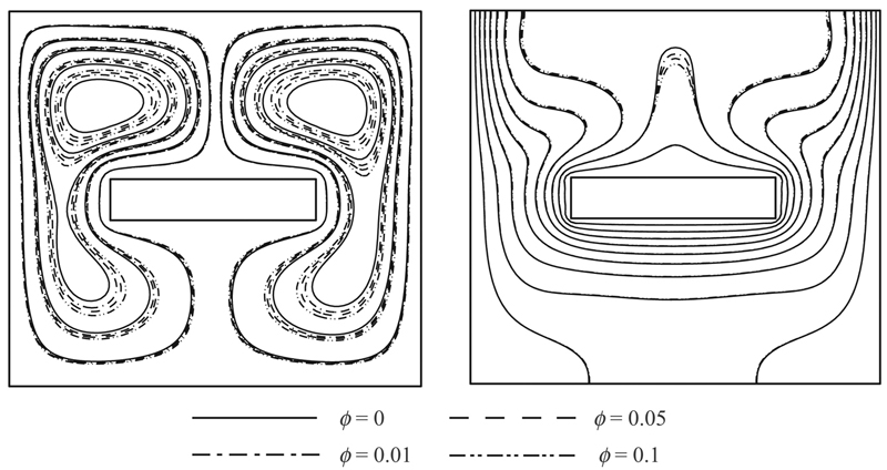
Figure 2.42 Streamline (left) and isotherm (right) for different values of Cu volume fraction when Ra = 105, H/t = 9, and Pr = 6.2.
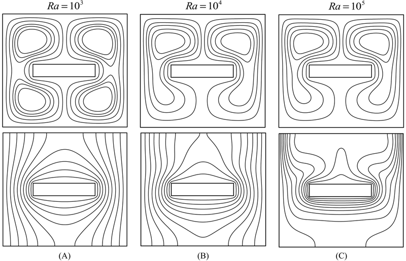
Figure 2.43 Streamlines (up) and isotherms (down) for (A) Ra = 103, (B) Ra = 104, and (C) Ra = 105 when, φ = 0.1, H/t = 9, and Pr = 6.2 (Cu–water case).
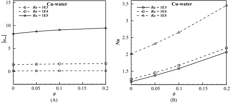
Figure 2.44 Effects of Ra and φ on (A) |ψmax|; (B) Nusselt number (Nu) for Cu–water nanofluid when H/t = 9.
It is observed that when φ increases from 0 to 0.1, both momentum and thermal boundary layer thicknesses increase. The enhancement in energy transport in the nanofluid with increasing volume fraction of nanoparticles increases velocity components of nanofluid. Thus, the absolute values of stream functions which indicate the strength of flow are enhanced with an increase of volume fraction of nanofluid. The sensitivity of thermal boundary layer thickness to volume fraction of nanoparticles is concerned with the increased thermal conductivity of the nanofluid. Moreover, thermal conductivity is accompanied by thermal diffusion in the nanofluid. The high value of thermal diffusivity causes decrease in the temperature gradients and consequently increases the boundary thickness as shown in Fig. 2.42. This increase in thermal boundary layer thickness reduces the Nusselt number. However, according to Eq. (2.120), the Nusselt number enhancement is due to increase in thermal conductivity ratio (knf/kf) because the reduction of temperature gradient for nanofluid (due to the presence of nanoparticles) is comparatively very less than increase in thermal conductivity ratio. Thus, this product leads to overall enhancement in Nusselt number with addition of nanoparticles. It is clear that with increasing Rayleigh number, the nanofluid isotherms move closer to the vertical walls and hence there are severe temperature gradients at the top corners. Ra, Rayleigh number, effectively embodies the relative contribution of thermal buoyancy force to viscous force in the nanofluid regime. It can be seen that increase in Ra leads to increase in the strength of flow, |ψmax| and the thermal boundary layer thickness decreases with a corresponding elevation in Nusselt number. At low Rayleigh number, the heat transfer is dominated by thermal conduction rather than thermal convection, and Nusselt number is very close to unity. However, by increasing Rayleigh number, the buoyancy forces increase substantially and they overcome the viscous forces so that the heat transfer is dominated by convection. Nusselt number is greater than unity at high Rayleigh number.
Fig. 2.45 shows the effect of the enclosure to internal body height ratio, H/t on streamline and isotherm distributions. With progressive reduction in the value of H/t, the size of the inner rectangle increases and the strength of the left eddies (vortices) (anticlockwise rotation) and right eddies (clockwise rotation) increases, as observed from the graph. The effects of Ra, H/t, and φ on |ψmax| and Nusselt number for (Cu–water case) are shown in Fig. 2.46A–B. It can be seen that as H/t increases, the distance between the cold wall and hot wall increases and this manifests in smaller heat transfer rates (lower Nusselt numbers). Fig. 2.46B shows that by increasing H/t, flow strength |ψmax| increases. Buoyancy force is also accentuated and dominates viscous force in the regime. Thus, for high values of H/t, the principal heat transfer mechanism is thermal convection. These changes are more pronounced for greater values of Rayleigh number.
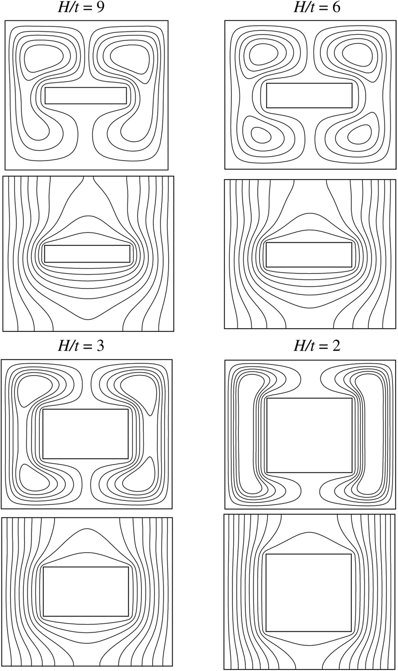
Figure 2.45 Streamlines (up) and isotherms (down) for different H/t when φ = 0.1, Ra = 104, and Pr = 6.2 (Cu–water case).
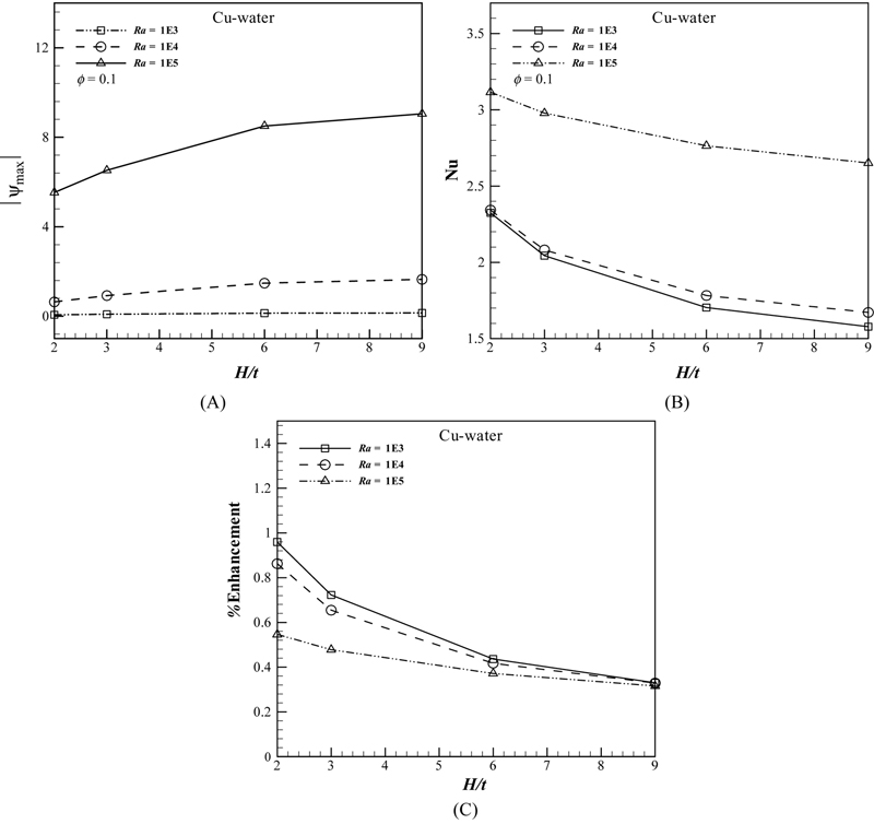
Figure 2.46 Effects of Ra, H/t, and φ on (A) |ψmax|; (B) Nusselt number for Cu–water nanofluid; (C) effects of H/t and Ra on ratio of enhancement of heat transfer due to addition of nanoparticles when Pr = 6.2 (Cu–water case).
The previous discussions indicate that generally heat transfer is enhanced in the regime with addition of nanoparticles. To estimate the enhancement of heat transfer between the case of φ = 0.1 and the pure fluid (base fluid) case, the enhancement is defined as
 (2.121)
Enhancement of heat transfer (φ = 0.1) is plotted versus H/t at different Rayleigh numbers in Fig. 2.46C. For the whole range of Rayleigh numbers, it is evident that enhancement of heat transfer generally decreases as H/t increases. Also, the percentage of heat transfer enhancement decreases with increasing of Rayleigh number for all values of H/t. Furthermore, by increasing H/t, the difference between percentages of heat transfer enhancement for various Rayleigh numbers also decreases. Additionally it is observed that the effect of nanoparticles is amplified at lower Rayleigh numbers than at higher Rayleigh numbers, a pattern which is attributable to the greater rate of heat transfer enhancement. This observation can be explained by noting that at low Rayleigh numbers the heat transfer is dominated by thermal conduction. Therefore, the addition of high thermal conductivity nanoparticles to the base fluid will serve to boost thermal conduction and make the enhancement more effective.
Fig. 2.47 shows the effects on Ra, H/t, Ω, and φ on dimensionless entropy generation number. According to these figures, dimensionless entropy generation number decreases with increase of Ω. This fact is consistent with the predictions of Eq. (2.108). This also makes physical sense since, as, Ω = Th/Tc−1 higher values of Ω imply a greater temperature difference (leading to higher heat transfer rates) and consequently an elevation in HTI values. Therefore, a decrease in <Ns>, according to  will result in an increase in the total entropy generation. For all values of Ra and H/t, it can be found that <Ns> increases with increasing φ. These changes are more pronounced for high values of Ra. Dimensionless entropy generation number increases as Ra increases, while it decreases as H/t increases.

Figure 2.47 Effect of Ra, H/t, Ω, and φ on dimensionless entropy generation number when H/t = 9 and Pr = 6.2 (Cu–water case).
Effect of the nanoparticle volume fraction (φ) for different types of nanofluid on |ψmax|, Nusselt number, and when H/t = 9 is shown in Tables 2.5 and 2.6. It emerges that streamlines, isotherms, flow strength |ψmax|, Nusselt number, and also dimensionless entropy generation are significantly modified by using different types of nanofluid. This means that the nanofluids have a great effect on the cooling and heating processes. Choosing silver as the nanoparticle leads to the maximum rate of heat transfer, max amount of <Ns> and max amount of |ψmax| although copper still performs well and is significantly less costly.
Table 2.5
Effect of the nanoparticle volume fraction on Nusselt number for different types of nanofluids when H/t = 9
| Nanoparticles | |||||
| Ra | φ | Cu | Ag | Al2O3 | TiO2 |
| 103 | 0.05 | 1.371959 | 1.372072 | 1.338052 | 1.203374 |
| 103 | 0.1 | 1.578062 | 1.578245 | 1.561584 | 1.503329 |
| 104 | 0.05 | 1.453494 | 1.453736 | 1.518718 | 1.418185 |
| 104 | 0.1 | 1.671232 | 1.671664 | 1.65474 | 1.593065 |
| 105 | 0.05 | 2.312486 | 2.315241 | 2.310522 | 2.265891 |
| 105 | 0.1 | 2.646458 | 2.651476 | 2.637898 | 2.540095 |

Table 2.6
Effect of the nanoparticle volume fraction on |ψmax| for different types of nanofluids when H/t = 9
| Nanoparticles | |||||
| Ra | φ | Cu | Ag | Al2O3 | TiO2 |
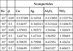
| 103 | 0.05 | 0.137081 | 0.14518 | 0.133852 | 0.133754 |
| 103 | 0.1 | 0.14697 | 0.160241 | 0.141644 | 0.140651 |
| 104 | 0.05 | 1.57803 | 1.59373 | 1.54046 | 1.52049 |
| 104 | 0.1 | 1.64716 | 1.67144 | 1.56052 | 1.55685 |
| 105 | 0.05 | 8.70855 | 8.79908 | 8.43554 | 8.42636 |
| 105 | 0.1 | 9.04689 | 9.09917 | 8.62427 | 8.60623 |
2.8. Two phase simulation of nanofluid flow and heat transfer using heatline analysis
2.8.1. Problem definition
The physical model and the corresponding triangular elements used in the present CVFEM program are shown in Fig. 2.48 [23]. The inner and outer walls are maintained at constant temperatures Th and Tc, respectively. The shape of inner cylinder profile is assumed to mimic the following pattern
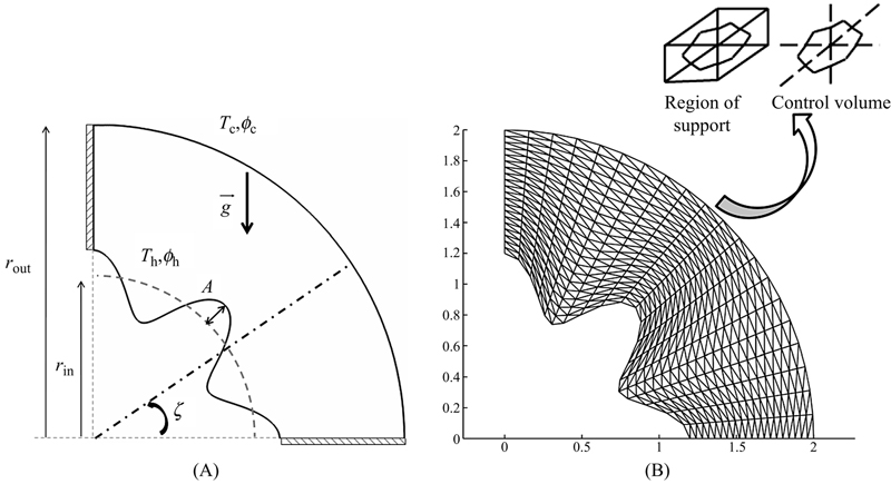
Figure 2.48 (A) Geometry and the boundary conditions; (B) the mesh of enclosure considered in this work.
 (2.122)
where rin is the base circle radius, rout is the radius of outer cylinder, A and N are amplitude and number of undulations, respectively, and ζ is the rotation angle. In this study A and N equal to 0.2 and 8, respectively.
The nanofluid’s density, ρ is
 (2.123)
where ρf is the base fluid’s density, Tc is a reference temperature, ρf0 is the base fluid’s density at the reference temperature, and β is the volumetric coefficient of expansion. Taking the density of base fluid as that of the nanofluid, as adopted by Yadav et al. [24], the density ρ in Eq. (2.123) thus becomes
ρ0 is the nanofluid’s density at the reference temperature.
The continuity, momentum under Boussinesq approximation, and energy equations for the laminar and steady state natural convection in a two-dimensional enclosure can be written in dimensional form as follows:
 (2.125)
 (2.126)
 (2.127)
 (2.128)
 (2.129)
Boundary conditions are
 (2.130)
The stream function and vorticity are defined as follows:
 (2.131)
The stream function satisfies the continuity Eq. (2.125). The vorticity equation is obtained by eliminating the pressure between the two momentum equations, that is, by taking y-derivative of Eq. (2.126) and subtracting from it the x-derivative of Eq. (2.127). Also the following nondimensional variables should be introduced:
 (2.132)
By using these dimensionless parameters the equations become [25]
 (2.133)
 (2.134)
 (2.135)
 (2.136)
where thermal Rayleigh number, the buoyancy ratio number, Prandtl number, the Brownian motion parameter, the thermophoretic parameter, and Lewis number of nanofluid are defined as: 
 ,
,  ,
,  ,
,  and
and  , respectively.
The Eq. (2.133) has been obtained using small temperature gradient in a dilute suspension of nanoparticles. The boundary conditions as shown in Fig. 2.48 are
 (2.137)
The values of vorticity on the boundary of the enclosure can be obtained using the stream function formulation and the known velocity conditions during the iterative solution procedure.
The local Nusselt number on the cold circular wall can be expressed as
 (2.138)
where n is the direction normal to the outer cylinder surface. The average number on the cold circular wall is evaluated as
 (2.139)
The heatlines are adequate tools for visualization and analysis of 2D convection heat transfer, through an extension of the heat flux line concept to include the advection terms. Heat function (H) is defined in terms of the energy equation as
 (2.140)
2.8.2. Effects of active parameters
In this study, CVFEM is applied to investigate natural convection heat transfer in an enclosure filled with nanofluid. Effects of thermal Rayleigh number (Ra = 103, 104, and 105), buoyancy ratio number (Nr = 0.1–4), and Lewis number (Le = 1, 2, 4, 6, and 8) on flow and heat transfer characteristics are examined. Brownian motion parameter of nanofluids (Nb = 0.5), thermophoretic parameter of nanofluids (Nt = 0.5), and Prandtl number (Pr = 10) are fixed. CVFEM has been used in this problem. In recent decade, several documents have been published by several authors as application of new numerical methods [26–40].
Comparison of the isotherms, streamlines, isoconcentration, and heatline contours for different values of thermal Rayleigh number is shown in Fig. 2.49. At Ra = 103 the conduction heat transfer mechanism is more pronounced. For this reason the isotherms are parallel to each other. As Ra increases, the distribution of isotherm contours increases. Streamline has two eddies within the enclosure of which the lower one is stronger. With increase of Ra, the role of convection in heat transfer becomes more significant. Also it can be seen that as Ra increases the distribution of isoconcentration contours increases. The heat flow within the enclosure is displayed using the heat function obtained from conductive heat fluxes (∂Θ/∂X, ∂Θ/∂Y) as well as convective heat fluxes (VΘ, UΘ). Heatlines emanate from hot regimes and end on cold regimes illustrating the path of heat flow. The domination of conduction heat transfer in low Rayleigh number can be observed from the heatline patterns as no passive area exists. The increase of Ra causes the clustering of heatlines from hot to the cold wall and generates passive heat transfer area in which heat is rotated without having significant effect on heat transfer between walls.
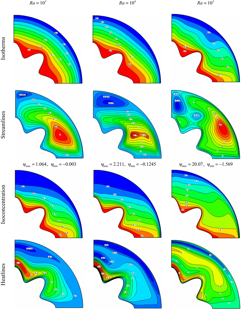
Figure 2.49 Comparison of the isotherms, streamlines, isoconcentration, and heatline contours for different values of thermal Rayleigh number when Nr = 4, Le = 8, Nt = Nb = 0.5, and Pr = 1/0.
Comparison of the isotherms, streamlines, isoconcentration, and heatline contours for different values of buoyancy ratio number is shown in Fig. 2.50. It should be mentioned that negative Nr values (opposing buoyancy forces) showed more complex and interesting flow patterns, such as multicells, which is worthy for presentation and discussion. So in this study results for positive Nr (aiding buoyancy forces), where the temperature- and species-induced buoyancy forces aid each other, are not considered. For Nr = 0, the species induced buoyancy force has no effect on flow; the flow is solely driven by the thermal buoyancy force. However, the effect of species-induced buoyancy increases as Nr value increases, and reaches a certain value, where the effect of thermally induced buoyancy becomes negligible in comparison to the solutal one. For small Nr value, the flow is mainly driven by the thermal buoyancy force. When Nr = 0.1, two upwelling plumes appear on the crests of the inner cylinder. A third plume appears above the outer circular cylinder with reverse direction owing to existing one counter clockwise eddy between two other clockwise eddies at this region. For Nr > 1 the flow is mainly driven by species concentration-induced buoyancy force. So as Nr increases thermal plumes disappear. The number of passive areas is increased with increase of solutal forces.
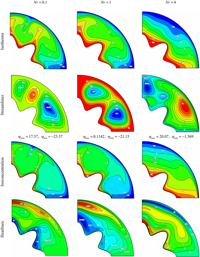
Figure 2.50 Comparison of the isotherms, streamlines, isoconcentration, and heatline contours for different values of buoyancy ratio number when Ra = 105, Le = 8, Nt = Nb = 0.5, and Pr = 10.
Comparison of the isotherms, streamlines, isoconcentration, and heatline contours for different values of Lewis number is shown in Fig. 2.51. When Le = 2, two equal eddies with same direction are observed. As Lewis number increases up to 8, these eddies are converted to four eddies. The mass flow is given by ψmax∼δsv, where the solutal boundary layer thickness is given by δs∼(RaLeNr)−1/4 and v∼(RaLeNr)1/2 so ψmax∼(RaLeNr)1/4. The solutal boundary layer, δs, becomes thinner by increasing either  or
or  or both. Heatlines are found to be more distorted as Le augments.
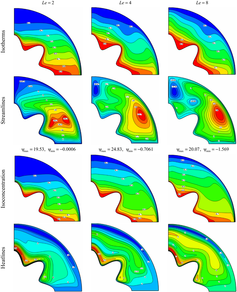
Figure 2.51 Comparison of the isotherms, streamlines, isoconcentration, and heatline contours for different values of Lewis number when Ra = 105, Nr = 4, Nt = Nb = 0.5, and Pr = 10.
Fig. 2.52 depicts the effects of thermal Rayleigh number, buoyancy ratio number, and Lewis number on local Nusselt number. A change in a flow structure has significant effect on the local Nusselt number. The number of extremum in the local Nusselt number profile corresponds to the number of thermal plume of cold wall. The occurrence of maxima for Nuloc is due to dense heatlines based on conductive heat transport occurring at those respective portions. For low values of Nr (Nr < 1) the maximum rate of heat transfer takes place at ζ = 90°, where the thermal boundary layer is thin. However, for Nr > 1, the reverse is true, that is, the rate of heat transfer is high at ζ = °. In fact, the trend reflects the physics of flow reversal as a function of Nr.
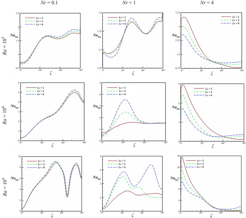
Figure 2.52 Effects of thermal Rayleigh number, buoyancy ratio number, and Lewis number on local Nusselt number at Nt = Nb = 0.5, and Pr = 10.
Fig. 2.53 shows the effects of thermal Rayleigh number, buoyancy ratio number, and Lewis number on average Nusselt number. As a general trend, the average Nusselt number decreases as Nr increases until it reaches a minimum value and then starts increasing. As Nr increases the effect of opposing buoyancy (species) increases, hence the net fluid flow driving force decreases. The Nuave reaches a minimum value when the strength of thermal buoyancy equals the species-induced buoyancy. The thermal boundary layer thickness differs from the species boundary layer thickness because Le is not at unity.

Figure 2.53 Effects of thermal Rayleigh number, buoyancy ratio number, and Lewis number on average Nusselt number at Nt = Nb = 0.5, and Pr = 10.
The minimum Nuave is obtained for buoyancy ratio number values (Nrcr) shifting slightly to higher Nr as Le increases. As the Le increases the species concentration boundary layer decreases in thickness compared with the thermal boundary layer thickness. Hence, the resulting species-induced force decreases as the Le increases and higher Nr is needed to compensate the decrease in the species concentration boundary layer. As expected the flow is dominated by species-induced buoyancy for Nr > Nrcr and rate of transport increases as Nr increases. The heat transfer increases with Le for Nr > Nrcr and decreases for Nr > Nrcr, for fixed Nr. Such a trend is a consequence of a separate scale on which the thermal and solutal effect acts and such a separate scale increases as the Le value increases. It is interesting to notice that the rate of decrease in Nuave is more prominent for Nr values between 0 and Nrcr compared with Nr greater than Nrcr. This can be explained by the fact that the results are obtained for Le ≥ 2; hence, the thermal boundary layer is thicker than the species concentration boundary layer.
..................Content has been hidden....................
You can't read the all page of ebook, please click here login for view all page.