
Chapter 2
Nanofluid Natural Convection Heat Transfer
Abstract
Natural convection heat transfer is an important phenomenon in engineering and industry with widespread applications in diverse fields, such as geophysics, solar energy, electronic cooling, and nuclear energy. Nanofluid can be used to enhance rate of heat transfer. Two common methods can be used to simulate nanofluid flow and heat transfer: single-phase model and two-phase model. Influence of active parameters has been examined.
Keywords
natural convection
nanofluid
CVFEM
LBM
single-phase model
two-phase model
heatline
2.1. CuO–water nanofluid hydrothermal analysis in a complex-shaped cavity
2.1.1. Problem definition and mathematical model
Fig. 2.1 depicts the geometry and boundary conditions [1]. The inner cylinder is hot and follows the following formula:

Figure 2.1 (A) Geometry and the boundary conditions with (B) the mesh of geometry considered in this work.
each parameters have been shown in Fig. 2.1.
2.1.1.1. Problem definition
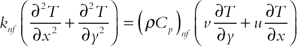
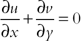
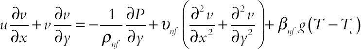
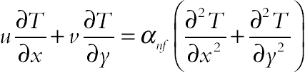
The governing equations for laminar CuO–water free convective heat transfer must be presented as
 (2.2)
(2.2)
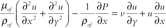 (2.3)
(2.3)
 (2.4)
(2.4)
 (2.5)
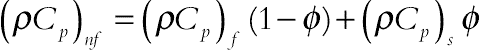
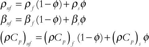
(2.5)(ρnf), (ρCp)nf, and βnf are defined as
 (2.7)
(2.7)
 (2.9)
(2.9)
 (2.10)
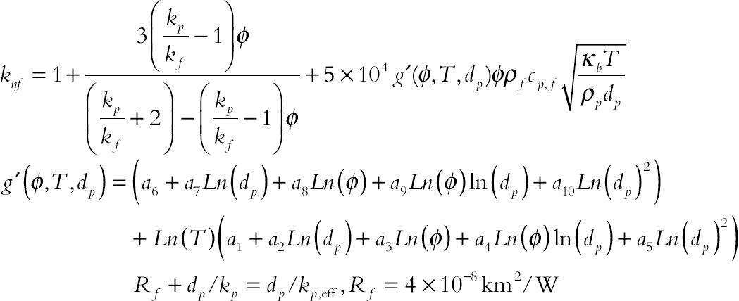
All needed coefficients and properties are illustrated in Tables 2.1 and 2.2 [2].
Table 2.1
The coefficient values of CuO–H2O nanofluid [2]
| Coefficient values | CuO–H2O |
| a1 | −26.593310846 |
| a2 | −0.403818333 |
| a3 | −33.3516805 |
| a4 | −1.915825591 |
| a5 | 6.42185846658E-02 |
| a6 | 48.40336955 |
| a7 | −9.787756683 |
| a8 | 190.245610009 |
| a9 | 10.9285386565 |
| a10 | −0.72009983664 |
Table 2.2
Thermo physical properties of water and nanoparticles [2]
| ρ (kg/m3) | Cp (j/kgk) | k (W/m.k) | β × 105 (K−1) | dp (nm) | σ (Ω·m)−1 | |
| H2O | 997.1 | 4179 | 0.613 | 21 | – | 0.05 |
| CuO | 6500 | 540 | 18 | 29 | 10-10 | 6500 |

Vorticity and stream function should be defined as
 (2.11)
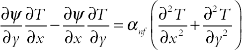
By removing pressure gradient source terms from Eqs. (2.3) and (2.4), the final form of equations can be obtained as
 (2.12)
 (2.13)
 (2.14)
Dimensionless parameters are as follows:
 (2.15)
Using the aforementioned formulae the governing equations change to
 (2.16)
 (2.17)
 (2.18)
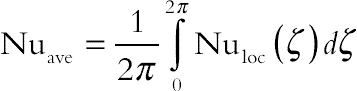
Rayleigh and Prandtl numbers are introduced as: Raf = gβf (Th−Tc) L3/(υfαf), Prf = υf/αf respectively. Nuloc and Nuave over the cold wall should be calculated as
 (2.19)
 (2.20)
2.1.1.2. Basic idea of CVFEM
Triangular elements are considered as the building block of the discretization using CVEM. Sample codes for control volume–based finite element method (CVFEM) exist in the appendix. The values of variables are approximated with linear interpolation within the elements. A control volume is created by joining the center of each element in the support to the midpoints of the element sides that pass through the central node i, which creates a close polygonal control volume (Fig. 2.2). To illustrate the solution procedure using the CVFEM, one can consider the general form of advection–diffusion equation for node i in integral form [3,4]:

Figure 2.2 The mesh of enclosure considered in this work.
 (2.21)
or point form
which can be represented by the system of CVFEM discrete equations as
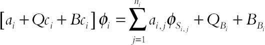 (2.23)
In the aforementioned equation, the as are the coefficients, the index (i, j) indicates the jth node in the support of node i, the index Si, j provides the node number of the jth node in the support, the Bs account for boundary conditions, and the Qs for source terms. For the selected triangular element which is shown in Fig. 2.3 this approximation without considering the source term leads to

Figure 2.3 A sample triangular element and its corresponding control volume.
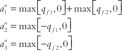
Using upwinding the advective coefficients, identified with the superscripts ( )u, are given by
 (2.25)
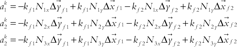
And the diffusion coefficients, identified with the superscripts ( )k, are given by
 (2.26)
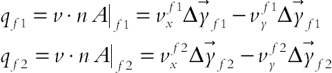
In Eq. (2.25) the volume flow across face 1 and 2 in the direction of the outward normal is
 (2.27)
The value of the diffusivity at the midpoint of face 1 can be obtained as
 (2.28)
and at the midpoint of face 2
 (2.29)
The velocity components at the midpoint of face 1 are as follows:
 (2.30)
And on face 2:
 (2.31)
These values can be used to update the ith support coefficients through the following equation:
 (2.32)
In Eq. (2.26), moving counterclockwise around node i, the signed distances are
 (2.33)
the derivatives of the shape functions are
 (2.34)
and the volume of the element is
 (2.35)
The obtained algebretic equations from the discretization procedure using CVFEM are solved by the Gauss–Seidel Method.
The boundary conditions for the present problem can be enforced using  and
and  as follows:
where φvalue is the prescribed value on the boundary and Ak is the length of the control volume surface on the boundary segment. The volume source terms can be applied to Eq. (2.22) as
 (2.39)
or after linearizing the as source term
2.1.2. Effects of active parameters
CuO–water hydrothermal analysis in a cavity with hot inner sinusoidal cylinder is studied via CVFEM. Different values for number of undulations (N = 2,3,5, and 6), nanoparticles volume fraction (φ = 0, 2, and 4%), and Rayleigh number (Ra = 103, 104, and 105) have been examined. Influence of nanoparticles on the velocity and temperature contours is illustrated in Fig. 2.4. The strength of flow enhances by adding nanoparticles in H2O. Furthermore, augmenting volume fraction of nanofluid causes the temperature to enhance. Influences of Rayleigh number and N on hydrothermal behavior are depicted in Figs. 2.5 and 2.6. |Ψmax| enhances with rise of buoyancy force.
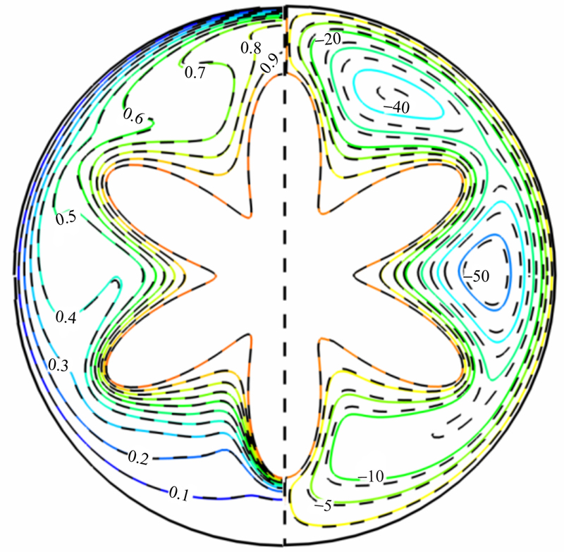
Figure 2.4 Comparison of the streamlines (left) and isotherms (right) contours between nanofluid (φ = 0.04) (––) and pure fluid (φ = 0) (- - -) for N = 6, A = 0.5 at Ra = 105 and Pr = 6.2.
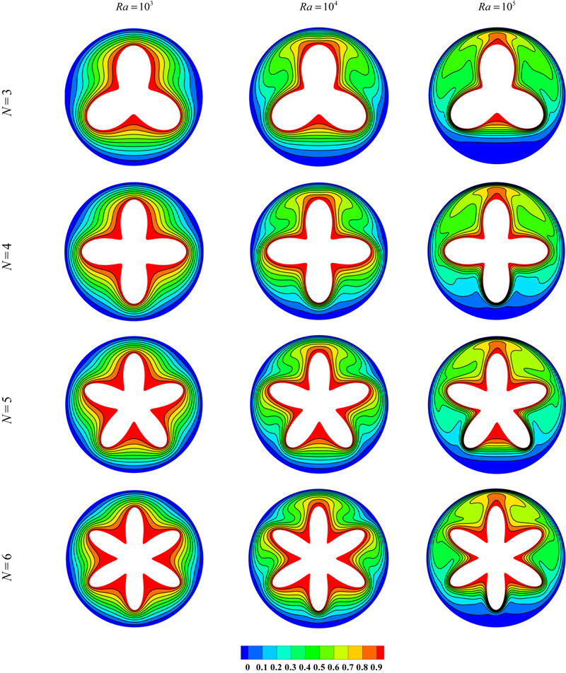
Figure 2.5 Comparison of the isotherms contours for different values of Rayleigh number (Ra) and number of undulations (N) at A = 0.5 and φ = 0.04.

Figure 2.6 Comparison of the streamlines contours for different values of Rayleigh number (Ra) and number of undulations (N) at A = 0.5 and φ = 0.04.
In low Reynolds number, augmenting in number of undulations causes |Ψmax| to enhance but at high Reynolds number this trend is not observed. Conduction heat transfer mode is dominant at low Reynolds number. So the isotherms are parallel to each other in those cases. Temperature gradient at the below of hot wall is higher than other places. For odd number of undulations, very small vortexes generate near the vertical centerline. The lower eddies are weaker than the upper ones because of smaller space for flow motion. As buoyancy forces augment thermal plumes generate on the hot wall. These plumes make isotherms to be denser and in turn temperature gradient enhances.
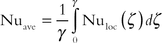
Effects of φ, Ra, and N on Nuloc and Nuave are depicted in Figs. 2.7 and 2.8, respectively. The average Nusselt number can be obtained according to following formula:
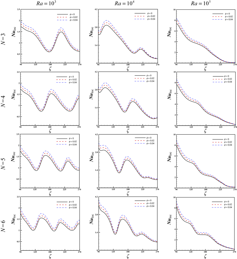
Figure 2.7 Effects of the nanoparticle volume fraction, number of undulations and Rayleigh number on local Nusselt number.
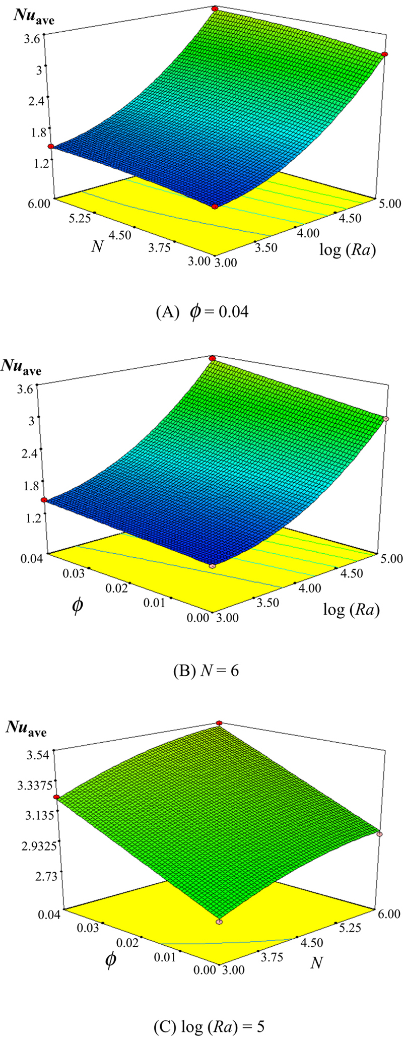
Figure 2.8 Effects of the nanoparticle volume fraction, number of undulations and Rayleigh number on average Nusselt number.
 (2.41)
The numbers of extremum in Nuloc are dependent on the number of undulation and thermal plumes. As ζ augments the conduction mechanism becomes dominant. So, Nuloc reduces with rise of ζ. Nusselt number enhances with rise of φ, Ra, and N.
2.2. Natural convection heat transfer in a nanofluid filled inclined L-shaped enclosure
2.2.1. Problem definition
The physical model along with the important geometrical parameters and the mesh of the enclosure used in the present CVFEM program are shown in Fig. 2.9 [5]. To assess the shape of inner circular and outer rectangular boundaries which consist of the right and top walls, a supper elliptic function can be used as follows:
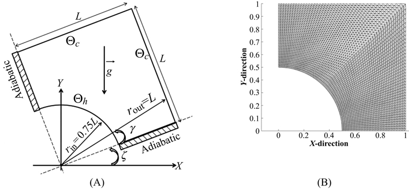
Figure 2.9 (A) Geometry and the boundary conditions with (B) the mesh of enclosure considered in this work.
 (2.42)
When a = b and n = 1 the geometry becomes a circle. As n increases from 1 the geometry would approach a rectangle for a ≠ b and square for a = b.
Dimensional governing equations are as follows:
 (2.43)
 (2.44)
 (2.45)
The boundary conditions as shown in Fig. 2.1A are
 (2.46)
The values of vorticity on the boundary of the enclosure can be obtained using the stream function formulation and the known velocity conditions during the iterative solution procedure. The local Nusselt number of the nanofluid along the hot wall can be expressed as
 (2.47)
where r is the radial direction. The average Nusselt number on hot circular wall is evaluated as
 (2.48)
2.2.2. Effects of active parameters
Natural convection heat transfer is an L-shape inclined enclosure filled with Cu–water nanofluid is investigated numerically using CVFEM. Calculations are made for various values of volume fraction of nanoparticles (φ = 0, 2, 4, and 6%), Rayleigh number (Ra = 103, 104, and 105), different inclination angles (ζ = −45°, 0°, and 45°), and constant Prandtl number (Pr = 6.2).
Comparison of the isotherms and streamlines contours for different values of Rayleigh numbers and inclination angles at φ = 0.06 is shown in Fig. 2.10. At Ra = 103 the isotherms are parallel to each other and take the shape of enclosure which is the main characteristic of conduction heat transfer mechanism. As Rayleigh number increases the isotherms become more distorted and the stream function values enhance which is due to the domination of convective heat transfer mechanism at higher Rayleigh numbers. At Ra = 103 and 104 the maximum value of stream function occurs at ζ = −45° while this maximum value is corresponding to ζ = 0° at Ra = 105. At ζ = 45° the temperature counters and streamlines are symmetric with respect to the vertical lines which pass through the corner of the enclosure. It is due to the existence of symmetric boundary condition and geometry of the cavity with respect to this line. At ζ = −45° and 0° increase of Rayleigh number causes the thermal boundary layer thickness on the hot circular wall decreases near the bottom wall of the enclosure hence it is predictable that the local Nusselt number obtains its minimum value at this area. The isotherms show that at Ra = 104, a thermal plume appears over the hot surface at γ = 45°. At this inclination angle when Ra increases up to 105 the thermal plum growth and impinges the hot fluid to the cold walls of the cavity.
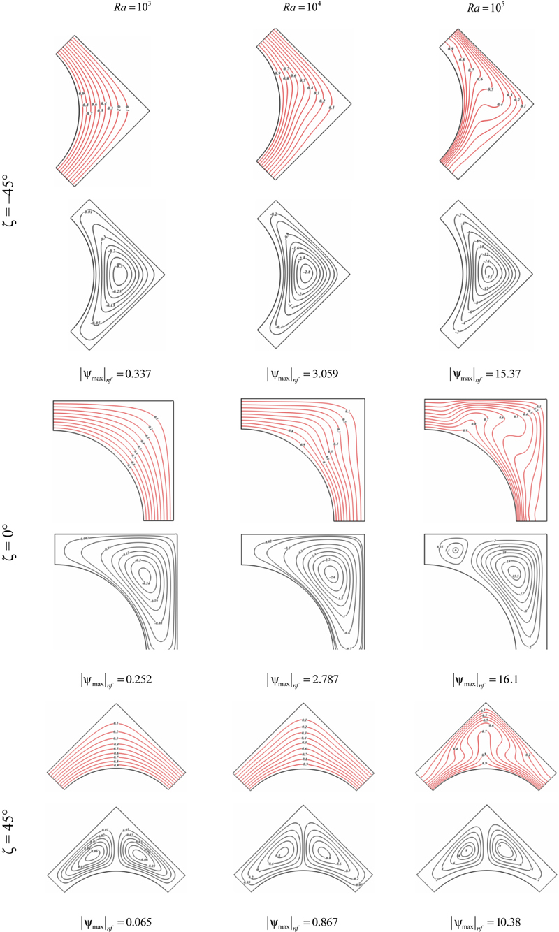
Figure 2.10 Comparison of the isotherms (up) and streamlines (down) contours for different values of Rayleigh numbers and inclined angles at φ = 0.06.
Fig. 2.11 shows the distribution of local Nusselt numbers along the surface of the inner circular wall for different inclination angles, Rayleigh numbers, and nanoparticle volume fractions. For all values of ζ, increasing the nanoparticle volume fraction and Rayleigh number lead to an increase in local Nusselt number. The sensitivity of thermal boundary layer thickness to volume fraction of nanoparticles is related to the increased thermal conductivity of the nanofluid. In fact, higher values of thermal conductivity are accompanied by higher values of thermal diffusivity. The high value of thermal diffusivity causes a drop in the temperature gradients and accordingly increases the boundary thickness. This increase in thermal boundary layer thickness reduces the Nusselt number; however, the Nusselt number is a multiplication of temperature gradient and the thermal conductivity ratio (conductivity of the nanofluid to the conductivity of the base fluid). As the reduction in temperature gradient due to the presence of nanoparticles is much smaller than thermal conductivity ratio an enhancement in Nusselt takes place by increasing the volume fraction of nanoparticles. At Ra = 103, because of domination conduction heat transfer mechanism, the distribution of the local Nusselt numbers along the surface of inner circular shows the symmetric shape. Also it can be found that as Rayleigh number increases the location of the minimum local Nusselt number approaches γ = 45°.
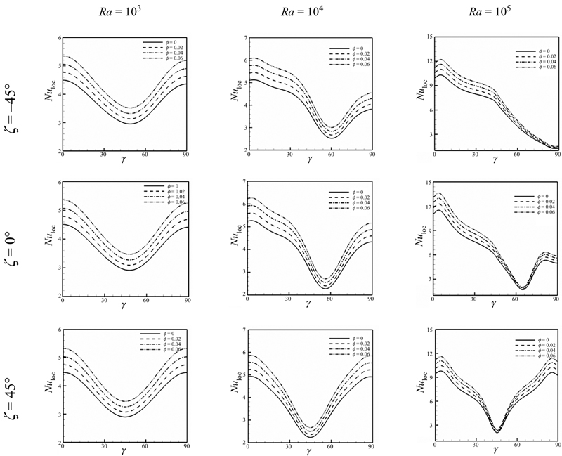
Figure 2.11 Effects of the nanoparticle volume fraction, Rayleigh number, and inclined angle for Cu–water nanofluids on local Nusselt number.
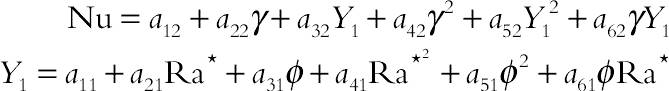
Fig. 2.12A shows the effects of Rayleigh number and inclination angle for Cu–water nanofluids on average Nusselt number. Effect of inclination angle on Nuave is more pronounced at higher Rayleigh number. At Ra = 104 the maximum and minimum average Nusselt number correspond to ζ = −45° and 45°, respectively, but opposite trend is observed for Ra = 105. The corresponding polynomial representation of such model for Nusselt number is as follows:
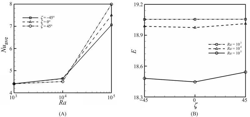
Figure 2.12 (A) Effects of Rayleigh number and inclination angle for Cu–water nanofluids on average Nusselt number at φ = 0.06; (B) effects of Rayleigh number and inclination angle for Cu–water nanofluids on the ratio of heat transfer enhancement due to addition of nanoparticles.
 (2.49)
Table 2.3
Constant coefficient for using Eq. (2.49)
| aij | i = 1 | i = 2 | i = 3 | i = 4 | i = 5 | i = 6 |
| j = 1 | 18.78013 | −8.82292 | −0.78209 | 1.26897 | −4.50225 | 3.891385 |
| j = 2 | 0.587531 | −0.85228 | 0.77581 | −0.01719 | 0.02018 | 0.198365 |

To estimate the enhancement of heat transfer between the case of φ = 0.06 and the pure fluid (base fluid) case, the enhancement is defined as
 (2.50)
The heat transfer enhancement ratio due to addition of nanoparticles for different values of ζ and Ra is shown in Fig. 2.12B. It can be found that the effect of nanoparticles is more pronounced at low Rayleigh number than at high Rayleigh number because of the greater enhancement rate. This observation can be explained by noting that at low Rayleigh number the heat transfer is dominant by conduction. Therefore, the addition of high thermal conductivity nanoparticles will increase the conduction and make the enhancement more effective. It is an interesting observation that the enhancement in heat transfer for at  is the same for all inclination angles. Also, for Ra = 104 and 105, minimum values of enhancement are obtained at ζ = 0°.
2.3. Natural convection heat transfer in a nanofluid filled enclosure with elliptic inner cylinder
2.3.1. Problem definition
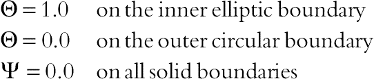
The schematic diagram and the mesh of the semiannulus enclosure used in the present CVFEM program are shown in Fig. 2.13 [6]. The system consists of a circular enclosure with radius of  , within which an inclined elliptic cylinder is located and rotates from γ = 0° to 90°. Th and Tc are the constant temperatures of the inner and outer cylinders, respectively, and Th > Tc. Setting a as the major axis and b as the minor axis of elliptic cylinder, the eccentricity (ɛ) for the inner cylinder is defined as

Figure 2.13 (A) Geometry and the boundary conditions with (B) the mesh of enclosure considered in this work.
In this section, for the inner ellipse, the eccentricity and the major axis are 0.9 and 0.8L, respectively.
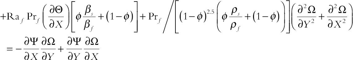
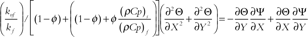
The flow is steady, two-dimensional, laminar, and incompressible. By using the Boussinesq approximation, the governing equations of heat transfer and fluid flow for nanofluid can be obtained as follows:
 (2.52)
 (2.53)
 (2.54)
 (2.55)
where the effective density (ρnf), the thermal expansion coefficient (βnf), and heat capacitance (ρCp)nf of the nanofluid are defined as
 (2.56)
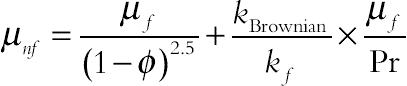
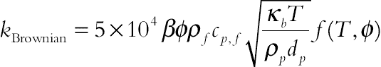
The Brownian motion has a significant impact on the effective thermal conductivity. Koo and Kleinstreuer [7] proposed that the effective thermal conductivity is composed of the particle’s conventional static part and a Brownian motion part. This 2-component thermal conductivity model takes into account the effects of particle size, particle volume fraction, and temperature dependence as well as types of particle and base fluid combinations.
 (2.58)
where kstatic is the static thermal conductivity based on Maxwell classical correlation. The enhanced thermal conductivity component generated by microscale convective heat transfer of a particle’s Brownian motion and affected by ambient fluid motion is obtained via simulating Stokes’ flow around a sphere (nanoparticle). By introducing two empirical functions (β and f) Koo [8] combined the interaction between nanoparticles in addition to the temperature effect in the model, leading to
 (2.59)
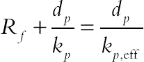
In recent years, there has been an increasing trend to emphasize the importance of the interfacial thermal resistance between nanoparticles and based fluids (see, e.g., Prasher et al. [9] and Jang and Choi [10]). The thermal interfacial resistance (Kapitza resistance) is believed to exist in the adjacent layers of the two different materials; the thin barrier layer plays a key role in weakening the effective thermal conductivity of the nanoparticle.
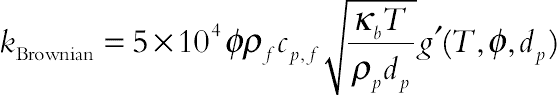
Li [11] revisited the model of Koo and Kleinstreuer [12] and combined β and f functions to develop a new g′ function which captures the influences of particle diameter, temperature, and volume fraction. The empirical g′-function depends on the type of nanofluid. Also, by introducing a thermal interfacial resistance Rf = 4 ×10⁻⁸ km2/W the original kp in Eq. (2.59) was replaced by a new kp,eff in the form:
 (2.60)
For different based fluids and different nanoparticles, the function should be different. Only water-based nanofluids are considered in the current study. For CuO–water nanofluids, this function follows the format:
 (2.61)
Finally, the KKL (Koo–Kleinstreuer–Li) correlation is written as
 (2.62)
Koo and Kleinstreuer [12] further investigated laminar nanofluid flow in micro heat sinks using the effective nanofluid thermal conductivity model they had established. For the effective viscosity due to micromixing in suspensions, they proposed
 (2.63)
where  is the viscosity of the nanofluid, as given originally by Brinkman.
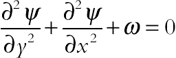
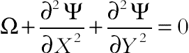
is the viscosity of the nanofluid, as given originally by Brinkman.The stream function and vorticity are defined as
 (2.64)
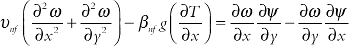
The stream function satisfies the continuity Eq. (2.52). The vorticity equation is obtained by eliminating the pressure between the two momentum equations, that is, by taking y-derivative of Eq. (2.53) and subtracting from it the x-derivative of Eq. (2.54). This gives
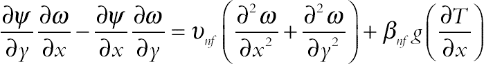 (2.65)
 (2.66)
 (2.67)
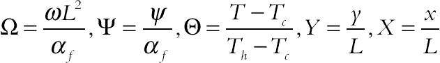
By introducing the following nondimensional variables:
 (2.68)
where L = rout. Using the dimensionless parameters, the equations now become
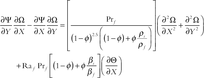 (2.69)
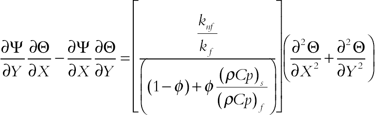 (2.70)
(2.71)where Raf = gβfL3(Th−Tc)/(αfυf) is the Rayleigh number for the base fluid and Prf = υf/αf is the Prandtl number for the base fluid. The boundary conditions as shown in Fig. 2.1 are
 (2.72)
The values of vorticity on the boundary of the enclosure can be obtained using the stream function formulation and the known velocity conditions during the iterative solution procedure.
The local Nusselt number of the nanofluid along the cold wall can be expressed as
(2.73)where r is the radial direction. The average Nusselt number on cold circular wall is evaluated as
 (2.74)
To estimate the enhancement of heat transfer between the case of φ = 0.04 and the pure fluid (base fluid) case, the enhancement is defined as
 (2.75)
2.3.2. Effects of active parameters
Natural convection heat transfer between a circular enclosure and an elliptic cylinder filled with nanofluid is investigated numerically using the CVFEM. The fluid in the enclosure is CuO–water nanofluid. Calculations are carried out for constant eccentricity (ɛ = 0.9), major axis (a = 0.8L) and Prandtl (Pr = 6.2) at different values of Rayleigh numbers (Ra = 103, 104, 105) and inclined angle of elliptic inner cylinder (γ = 0°, 30°, 60°, 90°), and volume fraction of nanoparticles (φ = 0, 2, and 4%).
Effects of adding nanoparticles on the streamlines and isotherms are shown in Fig. 2.14. As seen the absolute values of stream functions indicate that the strength of flow increases with increase in the volume fraction of nanofluid. Also it is obvious to say that adding nanoparticle leads to increase thermal boundary layer thickness so it decreases Nusselt number, while Nusselt number is a multiplication of temperature gradient and the thermal conductivity ratio. As the reduction in temperature gradient due to the presence of nanoparticles is much smaller than the thermal conductivity ratio, an enhancement in Nusselt occurs by adding nanoparticle.
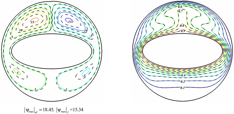
Figure 2.14 Comparison of the streamlines (left) and isotherms (right) contours between nanofluid (φ = 0.04) (––) and pure fluid (φ = 0) (- - -) for ɛ = 0.9, a = 0.8 L at Ra = 105 and Pr = 6.2.
Fig. 2.15 shows the isotherms and streamlines for different values of Ra and γ at φ = 0.04. At Ra = 103 the isotherms are parallel to each other and take the form of inner and outer walls and the stream function magnitude is relatively small which indicates the domination of conduction heat transfer mechanism. Increasing inclination angle leads to increase in the absolute value of maximum stream function (|Ψmax|) at this Rayleigh number. At γ = 0° the streamlines and isotherms are symmetric with respect to the vertical centerline of the enclosure. Each pair cells have two cells. The top vortex is stronger because at this area the hot surface is located beneath of the cold one which helps the flow circulation whereas the arrangement of the existence of cold wall under the hot cylinder at the bottom of the enclosure resists the flow circulation. As γ = 0° increases these two pair cells merge together and form two single cell different locations inside the enclosure. At γ = 90° again the streamlines pattern become symmetric with respect to the vertical centerline of the enclosure. At Ra = 104 the thermal plumbs start to appear over the hot elliptic cylinder. Besides, the stream function values start to grow which show that the convection heat transfer mechanism becomes comparable with conduction. At γ = 0° the temperature contour becomes stratified beneath the hot cylinder. With increase of γ to 30° a secondary vortex appears at the top of the enclosure and the thermal plumb slants to left because of more available space at this area. As the inclination angle of the inner cylinder increases, furthermore, this secondary vortex disappears and the streamlines show two main vortices in the enclosure. Also it can be found that effect of increasing inclination angle on |Ψmax| becomes less pronounced at γ = 30°. When Rayleigh number increases up to Ra = 105 isotherms are totally distorted at the top of the enclosure while it is stratified at the bottom of the enclosure which shows the heat transfer mechanism is dominated by convection. Thermal plumb generates which impinging the hot fluid to the cold wall of the enclosure. As seen the secondary vortex exists at γ = 30° and 60° which can slant the thermal plumb to left. Also, as seen in Fig. 2.15 maximum value of |Ψmax| occurs at γ = 60°.
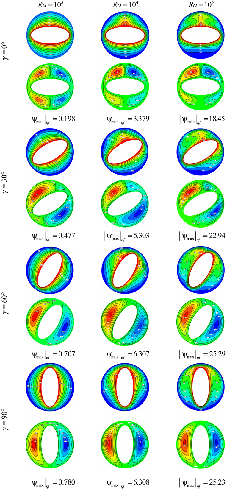
Figure 2.15 Isotherms (up) and streamlines (down) contours for different values of Ra and γ at φ = 0.04.
Fig. 2.16 shows the distribution of local Nusselt numbers along the surface of the outer circular wall for different inclination angle and Rayleigh number. As Rayleigh number increases the local Nusselt number increases due to increasing convection effect. At Ra = 103 the Nuloc profile is nearly symmetry with respect to the horizontal centerline. As Rayleigh number enhances (e.g., Ra = 104 and Ra = 105), the Nuloc profile is no longer symmetric and local Nusselt number is considerably small over the bottom wall of the enclosure. These local Nusselt number profiles are more complex due to the presence of thermal plume at the vicinity of the top wall of the enclosure.

Figure 2.16 Effects of the inclination angle and Rayleigh number on local Nusselt number when φ = 0.04.
Fig. 2.17 depicts the effects of the inclination angle and Rayleigh number on average Nusselt number. For all values of γ, the average Nusselt number increases with increase of Rayleigh number. As seen inclination angle has no significant effect on average Nusselt number at low Rayleigh number, while for higher values of Rayleigh number, increase in inclination angle leads to increase in average Nusselt number. Also, the corresponding polynomial representation of such model for Nusselt number is as follows:
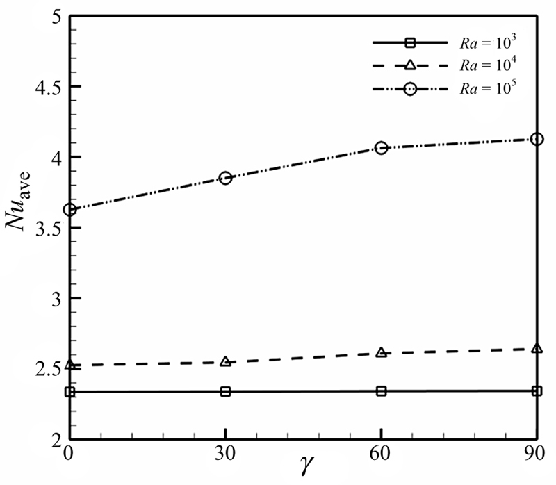
Figure 2.17 Effects of the inclination angle and Rayleigh number on average Nusselt number when φ = 0.04.
 (2.76)
Table 2.4
Constant coefficient for using Eq. (2.77)
| aij | i = 1 | i = 2 | i = 3 | i = 4 | i = 5 | i = 6 |
| j = 1 | 7.564525 | −3.38154 | −0.25235 | 0.506444 | 0.019843 | 2.008494 |
| j = 2 | 0.484538 | −0.31956 | 0.711765 | −0.04265 | 0.023808 | 0.1894 |

The heat transfer enhancement ratio due to addition of nanoparticles for different values of inclination angle and Rayleigh number is shown in Fig. 2.18. It can be found that the effect of nanoparticles is more pronounced at low Rayleigh number than at high Rayleigh number because of the greater enhancement rate. This observation can be explained by noting that at low Rayleigh number the heat transfer is dominant by conduction. Therefore, the addition of high thermal conductivity nanoparticles will increase the conduction and make the enhancement more effective. It is an interesting observation that the enhancement in heat transfer for Ra = 103 is the same for all inclination angles. At Ra = 104 the maximum heat transfer enhancement ratio is obtained at γ = 30°. At high Rayleigh number (Ra = 105), at first the percentage of heat transfer enhancement decreases and then increases. At this Rayleigh number the minimum heat transfer enhancement ratio occurs at γ = 90°.
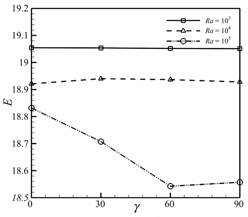
Figure 2.18 Effects of the inclination angle and Rayleigh number on the ratio of heat transfer enhancement due to addition of nanoparticles when Pr = 6.2.
..................Content has been hidden....................
You can't read the all page of ebook, please click here login for view all page.