Search in book...
Toggle Font Controls
Create new playlist

Name your new playlist

Playlist description (optional)
Sign In

Email address

Password

Forgot Password?

or

Continue with Facebook

Continue with Google
Sign Up

Full Name

Email address

Confirm Email Address

Password

or

Continue with Facebook

Continue with Google

Chapter 3

Nanofluid Forced Convection Heat Transfer

Abstract

Forced convection is a mechanism or a type of transport in which fluid motion is generated by an external source (such as a pump, fan, suction device, etc.). It should be considered as one of the main methods of useful heat transfer, as significant amounts of heat energy can be transported very efficiently. Nanofluid can be used as a working fluid to the improve rate of heat transfer. In this chapter, some applications of nanofluid forced convective heat transfer are presented.

Keywords

forced convection

nanofluid

numerical method

semianalytical method

3.1. Effect of nonuniform magnetic field on forced convection heat transfer of Fe₃O₄-water nanofluid

3.1.1. Problem definition

The schematic diagram and the mesh of the semiannulus enclosure used in the present CVFEM program are shown in Fig. 3.1 [1]. The inner wall is maintained at constant temperatures T_h and the other walls are maintained at constant temperature T_c (T_h > T_c). For the expression of the magnetic field strength, it can be considered that the magnetic source represents a magnetic wire placed vertically to the x–y plane at the point

(\bar{a}, \bar{b})

$(\bar{a}, \bar{b})$

. The components of the magnetic field intensity

(\bar{H_{x}}, \bar{H_{y}})

$(\bar{H_{x}}, \bar{H_{y}})$

and the magnetic field strength

(\bar{H_{x}})

$(\bar{H_{x}})$

can be considered as Ref. [2]:

Figure 3.1 (A) Geometry and the boundary conditions and (B) the mesh of enclosure considered in this work.

$\bar{H_{x}} = \frac{γ^{'}}{2 π} \frac{1}{{(x - \bar{a})}^{2} + {(y - \bar{b})}^{2}} (y - \bar{b})$ $\bar{H_{x}} = \frac{γ^{'}}{2 π} \frac{1}{{(x - \bar{a})}^{2} + {(y - \bar{b})}^{2}} (y - \bar{b})$

(3.1)

$\bar{H_{y}} = - \frac{γ^{'}}{2 π} \frac{1}{{(x - \bar{a})}^{2} + {(y - \bar{b})}^{2}} (x - \bar{a})$ $\bar{H_{y}} = - \frac{γ^{'}}{2 π} \frac{1}{{(x - \bar{a})}^{2} + {(y - \bar{b})}^{2}} (x - \bar{a})$

(3.2)

$\bar{H} = \sqrt{{\bar{H}}_{x}^{2} + {\bar{H}}_{y}^{2}} = \frac{γ^{'}}{2 π} \frac{1}{\sqrt{{(x - \bar{a})}^{2} + {(y - \bar{b})}^{2}}}$ $\bar{H} = \sqrt{{\bar{H}}_{x}^{2} + {\bar{H}}_{y}^{2}} = \frac{γ^{'}}{2 π} \frac{1}{\sqrt{{(x - \bar{a})}^{2} + {(y - \bar{b})}^{2}}}$

(3.3)

where γ′ the magnetic field strength at the source (of the wire) and

(\bar{a}, \bar{b})

$(\bar{a}, \bar{b})$

is the position where the source is located. The contours of the magnetic field strength are shown in Fig. 3.2. In this study magnetic source is located at (−0.01 cols, 0.5 rows). The lower wall is Lid driven with velocity of U_Lid. In this study γ is equal to 45°.

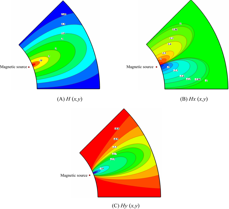
Figure 3.2 Contours of the (A) magnetic field strength H; (B) magnetic field intensity component in x direction, Hx; (C) magnetic field intensity component in y direction, Hy.

The flow is two dimensional, laminar, and incompressible. The magnetic Reynolds number is assumed to be small, so that the induced magnetic field can be neglected compared to the applied magnetic field. The flow is considered to be steady, two dimensional, and laminar. Using the Boussinesq approximation, the governing equations of heat transfer and fluid flow for nanofluid can be obtained as follows:

$\frac{\partial u}{\partial x} + \frac{\partial v}{\partial y} = 0$ $\frac{\partial u}{\partial x} + \frac{\partial v}{\partial y} = 0$

(3.4)

$ρ_{nf} (u \frac{\partial u}{\partial x} + v \frac{\partial u}{\partial y}) = - \frac{\partial P}{\partial x} + μ_{nf} (\frac{\partial^{2} u}{\partial x^{2}} + \frac{\partial^{2} u}{\partial y^{2}}) - σ_{nf} B_{y}^{2} u + σ_{nf} B_{x} B_{y} v$ $ρ_{nf} (u \frac{\partial u}{\partial x} + v \frac{\partial u}{\partial y}) = - \frac{\partial P}{\partial x} + μ_{nf} (\frac{\partial^{2} u}{\partial x^{2}} + \frac{\partial^{2} u}{\partial y^{2}}) - σ_{nf} B_{y}^{2} u + σ_{nf} B_{x} B_{y} v$

(3.5)

$ρ_{nf} (u \frac{\partial v}{\partial x} + v \frac{\partial v}{\partial y}) = - \frac{\partial P}{\partial y} + μ_{nf} (\frac{\partial^{2} v}{\partial x^{2}} + \frac{\partial^{2} v}{\partial y^{2}}) - σ_{nf} B_{x}^{2} v + σ_{nf} B_{x} B_{y} u$ $ρ_{nf} (u \frac{\partial v}{\partial x} + v \frac{\partial v}{\partial y}) = - \frac{\partial P}{\partial y} + μ_{nf} (\frac{\partial^{2} v}{\partial x^{2}} + \frac{\partial^{2} v}{\partial y^{2}}) - σ_{nf} B_{x}^{2} v + σ_{nf} B_{x} B_{y} u$

(3.6)

$\begin{array}{l} {(ρ C_{p})}_{nf} (u \frac{\partial T}{\partial x} + v \frac{\partial T}{\partial y}) = k_{nf} (\frac{\partial^{2} T}{\partial x^{2}} + \frac{\partial^{2} T}{\partial y^{2}}) + σ_{nf} {(u B_{y} - v B_{x})}^{2} \\ - μ_{0} T \frac{\partial M}{\partial T} (u \frac{\partial \bar{H}}{\partial x} + v \frac{\partial \bar{H}}{\partial y}) + μ_{nf} \{2 {(\frac{\partial u}{\partial x})}^{2} + 2 {(\frac{\partial v}{\partial y})}^{2} + {(\frac{\partial u}{\partial y} + \frac{\partial v}{\partial x})}^{2}\} \end{array}$ $\begin{array}{l} {(ρ C_{p})}_{nf} (u \frac{\partial T}{\partial x} + v \frac{\partial T}{\partial y}) = k_{nf} (\frac{\partial^{2} T}{\partial x^{2}} + \frac{\partial^{2} T}{\partial y^{2}}) + σ_{nf} {(u B_{y} - v B_{x})}^{2} \\ - μ_{0} T \frac{\partial M}{\partial T} (u \frac{\partial \bar{H}}{\partial x} + v \frac{\partial \bar{H}}{\partial y}) + μ_{nf} \{2 {(\frac{\partial u}{\partial x})}^{2} + 2 {(\frac{\partial v}{\partial y})}^{2} + {(\frac{\partial u}{\partial y} + \frac{\partial v}{\partial x})}^{2}\} \end{array}$

(3.7)

The terms

- σ_{nf} B_{y}^{2} u + σ_{nf} B_{x} B_{y} v

$- σ_{nf} B_{y}^{2} u + σ_{nf} B_{x} B_{y} v$

and

- σ_{nf} B_{x}^{2} v + σ_{nf} B_{x} B_{y} u

$- σ_{nf} B_{x}^{2} v + σ_{nf} B_{x} B_{y} u$

appearing in Eqs. (3.5) and (3.6), respectively, represent the Lorentz force per unit volume toward the x and y directions and arise due to the electrical conductivity of the fluid. These two terms are known in magnetohydrodynamics (MHD). The term

μ_{0} T \frac{\partial M}{\partial T} (u \frac{\partial \bar{H}}{\partial x} + v \frac{\partial \bar{H}}{\partial y})

$μ_{0} T \frac{\partial M}{\partial T} (u \frac{\partial \bar{H}}{\partial x} + v \frac{\partial \bar{H}}{\partial y})$

in Eq. (3.7) represents the thermal power per unit volume due to the magnetocaloric effect. Also the term σ_nf (uB_y − vB_x)² in Eq. (3.7) represents the Joule heating. For the variation of the magnetization M, with the magnetic field intensity

\bar{H}

$\bar{H}$

and temperature T, the following relation derived experimentally in Ref. [2] is considered:

$M = K^{'} \bar{H} ({T^{'}}_{c} - T)$ $M = K^{'} \bar{H} ({T^{'}}_{c} - T)$

(3.8)

where K′ is a constant and

{T^{'}}_{c}

${T^{'}}_{c}$

is the Curie temperature.

In the earlier equations, μ₀ is the magnetic permeability of vacuum (4π × 10⁻⁷ Tm/A),

\bar{H}

$\bar{H}$

is the magnetic field strength,

\bar{B}

$\bar{B}$

is the magnetic induction

(\bar{B} = μ_{0} \bar{H})

$(\bar{B} = μ_{0} \bar{H})$

, and the bar above the quantities denotes that they are dimensional. The effective density (ρ_nf) and heat capacitance

{(ρ C_{p})}_{nf}

${(ρ C_{p})}_{nf}$

of the nanofluid are defined as:

$ρ_{nf} = ρ_{f} (1 - φ) + ρ_{s} φ$ $ρ_{nf} = ρ_{f} (1 - φ) + ρ_{s} φ$

(3.9)

${(ρ C_{p})}_{nf} = {(ρ C_{p})}_{f} (1 - φ) + {(ρ C_{p})}_{s} φ$ ${(ρ C_{p})}_{nf} = {(ρ C_{p})}_{f} (1 - φ) + {(ρ C_{p})}_{s} φ$

(3.10)

where ɸ is the solid volume fraction of nanoparticles. Thermal diffusivity of the nanofluid is

$α_{nf} = \frac{k_{nf}}{{(ρ C_{p})}_{nf}}$ $α_{nf} = \frac{k_{nf}}{{(ρ C_{p})}_{nf}}$

(3.11)

The dynamic viscosity of the nanofluid given by Sheikholeslami et al. [1] is

$μ_{nf} = \frac{μ_{f}}{{(1 - φ)}^{2.5}}$ $μ_{nf} = \frac{μ_{f}}{{(1 - φ)}^{2.5}}$

(3.12)

The effective thermal conductivity of the nanofluid can be approximated as [1]:

$\frac{k_{nf}}{k_{f}} = \frac{k_{s} + 2 k_{f} - 2 φ (k_{f} - k_{s})}{k_{s} + 2 k_{f} + φ (k_{f} - k_{s})}$ $\frac{k_{nf}}{k_{f}} = \frac{k_{s} + 2 k_{f} - 2 φ (k_{f} - k_{s})}{k_{s} + 2 k_{f} + φ (k_{f} - k_{s})}$

(3.13)

and the effective electrical conductivity of nanofluid was presented by Sheikholeslami et al. [1] as:

$\frac{σ_{nf}}{σ_{f}} = 1 + \frac{3 (\frac{σ_{s}}{σ_{f}} - 1) φ}{(\frac{σ_{s}}{σ_{f}} + 2) - (\frac{σ_{s}}{σ_{f}} - 1) φ}$ $\frac{σ_{nf}}{σ_{f}} = 1 + \frac{3 (\frac{σ_{s}}{σ_{f}} - 1) φ}{(\frac{σ_{s}}{σ_{f}} + 2) - (\frac{σ_{s}}{σ_{f}} - 1) φ}$

(3.14)

The stream function and vorticity are defined as:

$u = \frac{\partial ψ}{\partial y}, v = - \frac{\partial ψ}{\partial x}, ω = \frac{\partial v}{\partial x} - \frac{\partial u}{\partial y}$ $u = \frac{\partial ψ}{\partial y}, v = - \frac{\partial ψ}{\partial x}, ω = \frac{\partial v}{\partial x} - \frac{\partial u}{\partial y}$

(3.15)

The stream function satisfies the continuity Eq. (3.4). The vorticity equation is obtained by eliminating the pressure between the two momentum equations, that is, by taking y-derivative of Eq. (3.6) and subtracting from it the x-derivative of Eq. (3.5). By introducing the following nondimensional variables:

$\begin{array}{l} X = \frac{x}{L}, Y = \frac{y}{L}, Ω = \frac{ω L}{U_{L i d}}, Ψ = \frac{ψ}{L U_{L i d}}, Θ = \frac{T - T_{c}}{T_{h} - T_{c}}, U = \frac{u}{U_{L i d}}, V = \frac{v}{U_{L i d}}, \\ H = \frac{\bar{H}}{\bar{H_{0}}}, H_{x} = \frac{\bar{H_{x}}}{\bar{H_{0}}}, H_{y} = \frac{\bar{H_{y}}}{\bar{H_{0}}} \end{array}$ $\begin{array}{l} X = \frac{x}{L}, Y = \frac{y}{L}, Ω = \frac{ω L}{U_{L i d}}, Ψ = \frac{ψ}{L U_{L i d}}, Θ = \frac{T - T_{c}}{T_{h} - T_{c}}, U = \frac{u}{U_{L i d}}, V = \frac{v}{U_{L i d}}, \\ H = \frac{\bar{H}}{\bar{H_{0}}}, H_{x} = \frac{\bar{H_{x}}}{\bar{H_{0}}}, H_{y} = \frac{\bar{H_{y}}}{\bar{H_{0}}} \end{array}$

(3.16)

where in Eq. (3.17) $\bar{H_{0}} = \bar{H} (\bar{a}, 0) = \frac{γ}{2 π | b |}$ $\bar{H_{0}} = \bar{H} (\bar{a}, 0) = \frac{γ}{2 π | b |}$ and L = r_out − r_in = r_in. Using the dimensionless parameters, the equations now become:

$\begin{array}{l} \frac{\partial Ψ}{\partial Y} \frac{\partial Ω}{\partial X} - \frac{\partial Ψ}{\partial X} \frac{\partial Ω}{\partial Y} = \frac{1}{Re} [\frac{μ_{nf} / μ_{f}}{ρ_{nf} / ρ_{f}}] (\frac{\partial^{2} Ω}{\partial X^{2}} + \frac{\partial^{2} Ω}{\partial Y^{2}}) \\ - \frac{H a^{2}}{R e} [\frac{σ_{nf} / σ_{f}}{ρ_{nf} / ρ_{f}}] \\ \times \{\frac{\partial V}{\partial X} H_{x}^{2} + V (2 H_{x} \frac{\partial H_{x}}{\partial X}) - \frac{\partial U}{\partial X} H_{x} H_{y} - U \frac{\partial H_{x}}{\partial X} H_{y} - U \frac{\partial H_{y}}{\partial X} H_{x} \\ - \frac{\partial U}{\partial Y} H_{y}^{2} - U (2 H_{y} \frac{\partial H_{y}}{\partial Y}) + \frac{\partial V}{\partial Y} H_{x} H_{y} + V \frac{\partial H_{x}}{\partial Y} H_{y} + V \frac{\partial H_{y}}{\partial Y} H_{x}\} \end{array}$ $\begin{array}{l} \frac{\partial Ψ}{\partial Y} \frac{\partial Ω}{\partial X} - \frac{\partial Ψ}{\partial X} \frac{\partial Ω}{\partial Y} = \frac{1}{Re} [\frac{μ_{nf} / μ_{f}}{ρ_{nf} / ρ_{f}}] (\frac{\partial^{2} Ω}{\partial X^{2}} + \frac{\partial^{2} Ω}{\partial Y^{2}}) \\ - \frac{H a^{2}}{R e} [\frac{σ_{nf} / σ_{f}}{ρ_{nf} / ρ_{f}}] \\ \times \{\frac{\partial V}{\partial X} H_{x}^{2} + V (2 H_{x} \frac{\partial H_{x}}{\partial X}) - \frac{\partial U}{\partial X} H_{x} H_{y} - U \frac{\partial H_{x}}{\partial X} H_{y} - U \frac{\partial H_{y}}{\partial X} H_{x} \\ - \frac{\partial U}{\partial Y} H_{y}^{2} - U (2 H_{y} \frac{\partial H_{y}}{\partial Y}) + \frac{\partial V}{\partial Y} H_{x} H_{y} + V \frac{\partial H_{x}}{\partial Y} H_{y} + V \frac{\partial H_{y}}{\partial Y} H_{x}\} \end{array}$

(3.17)

$\begin{array}{l} \frac{\partial Ψ}{\partial Y} \frac{\partial Θ}{\partial X} - \frac{\partial Ψ}{\partial X} \frac{\partial Θ}{\partial Y} = \frac{1}{P r R e} (\frac{k_{nf}}{k_{f}}) / (\frac{{(ρ C_{p})}_{nf}}{{(ρ C_{p})}_{f}}) (\frac{\partial^{2} Θ}{\partial X^{2}} + \frac{\partial^{2} Θ}{\partial Y^{2}}) \\ + {H a^{2} \frac{E c}{R e} (\frac{σ_{nf}}{σ_{f}}) / (\frac{{(ρ C_{p})}_{nf}}{{(ρ C_{p})}_{f}}) \{U H_{y} - V H_{x}\}}^{2} \\ + M n_{F} E c \frac{{(ρ C_{p})}_{f}}{{(ρ C_{p})}_{nf}} \{U \frac{\partial H}{\partial X} + V \frac{\partial H}{\partial Y}\} H (ɛ_{1} + Θ) \\ + \frac{E c}{R e} (\frac{μ_{nf}}{μ_{f}}) / (\frac{{(ρ C_{p})}_{nf}}{{(ρ C_{p})}_{f}}) \{2 {(\frac{\partial U}{\partial X})}^{2} + 2 {(\frac{\partial V}{\partial Y})}^{2} + {(\frac{\partial U}{\partial Y} + \frac{\partial V}{\partial X})}^{2}\} \end{array}$ $\begin{array}{l} \frac{\partial Ψ}{\partial Y} \frac{\partial Θ}{\partial X} - \frac{\partial Ψ}{\partial X} \frac{\partial Θ}{\partial Y} = \frac{1}{P r R e} (\frac{k_{nf}}{k_{f}}) / (\frac{{(ρ C_{p})}_{nf}}{{(ρ C_{p})}_{f}}) (\frac{\partial^{2} Θ}{\partial X^{2}} + \frac{\partial^{2} Θ}{\partial Y^{2}}) \\ + {H a^{2} \frac{E c}{R e} (\frac{σ_{nf}}{σ_{f}}) / (\frac{{(ρ C_{p})}_{nf}}{{(ρ C_{p})}_{f}}) \{U H_{y} - V H_{x}\}}^{2} \\ + M n_{F} E c \frac{{(ρ C_{p})}_{f}}{{(ρ C_{p})}_{nf}} \{U \frac{\partial H}{\partial X} + V \frac{\partial H}{\partial Y}\} H (ɛ_{1} + Θ) \\ + \frac{E c}{R e} (\frac{μ_{nf}}{μ_{f}}) / (\frac{{(ρ C_{p})}_{nf}}{{(ρ C_{p})}_{f}}) \{2 {(\frac{\partial U}{\partial X})}^{2} + 2 {(\frac{\partial V}{\partial Y})}^{2} + {(\frac{\partial U}{\partial Y} + \frac{\partial V}{\partial X})}^{2}\} \end{array}$

(3.18)

$\frac{\partial^{2} Ψ}{\partial X^{2}} + \frac{\partial^{2} Ψ}{\partial Y^{2}} = - Ω$ $\frac{\partial^{2} Ψ}{\partial X^{2}} + \frac{\partial^{2} Ψ}{\partial Y^{2}} = - Ω$

(3.19)

where

R e = \frac{ρ_{f} L U_{L i d}}{μ_{f}}, H a = L H_{0} μ_{0} \sqrt{σ_{f} / μ_{f}}, ɛ_{1} = T_{1} / ∆ T

$R e = \frac{ρ_{f} L U_{L i d}}{μ_{f}}, H a = L H_{0} μ_{0} \sqrt{σ_{f} / μ_{f}}, ɛ_{1} = T_{1} / ∆ T$

and

E c = (ρ_{f} U_{L i d}^{2}) / [{(ρ C_{p})}_{f} ∆ T]

$E c = (ρ_{f} U_{L i d}^{2}) / [{(ρ C_{p})}_{f} ∆ T]$

are the Reynolds number, Hartmann number, temperature number, and Eckert number for the base fluid, respectively. The thermophysical properties of the nanofluid are given in Table 3.1 [1].

The boundary conditions as shown in Fig. 3.1 are:

Table 3.1

Thermophysical properties of water and nanoparticles [1]

	ρ (kg/m³)	C_p (J/kg·K)	k (W/m·K)	β × 10⁵ (K⁻¹)	d_p (nm)	σ (Ω·m)⁻¹
Pure water	997.1	4,179	0.613	21	—	0.05
Fe₃O₄	5,200	670	6	1.3	47	25,000

$\begin{array}{l} Θ = 1.0 & on the inner circular boundary \\ Θ = 0.0 & on the other walls \end{array}$ $\begin{array}{l} Θ = 1.0 & on the inner circular boundary \\ Θ = 0.0 & on the other walls \end{array}$

(3.20)

The values of vorticity on the boundary of the enclosure can be obtained using the stream function formulation and the known velocity conditions during the iterative solution procedure.

The local Nusselt number of the nanofluid along the hot wall can be expressed as:

$N u_{loc} = (\frac{k_{nf}}{k_{f}}) \frac{\partial Θ}{\partial r}$ $N u_{loc} = (\frac{k_{nf}}{k_{f}}) \frac{\partial Θ}{\partial r}$

(3.21)

where r is the radial direction. The average Nusselt number on the hot circular wall is evaluated as:

$N u_{ave} = \frac{1}{γ} \int_{0}^{γ} N u_{loc} (ζ) d ζ$ $N u_{ave} = \frac{1}{γ} \int_{0}^{γ} N u_{loc} (ζ) d ζ$

(3.22)

To estimate the enhancement of heat transfer between the case of ɸ = 0.04 and the pure fluid (base fluid) case, the heat transfer enhancement is defined as:

$E n = \frac{N u (φ = 0.04) - N u (basefluid)}{N u (basefluid)} \times 100$ $E n = \frac{N u (φ = 0.04) - N u (basefluid)}{N u (basefluid)} \times 100$

(3.23)

3.1.2. Effects of active parameters

Forced convection heat transfer of ferrofluid in the presence of variable magnetic field is investigated using CVFEM. The working fluid is Fe₃O₄-water nanofluid. Calculations are made for various values of volume fraction of nanoparticles (ɸ = 0 and 4%), Reynolds number (Re = 10, 100, and 1000), and Hartmann number (Ha = 0, 5, 10, and 20). In all calculations, the Prandtl number (Pr), temperature number (ɛ₁) and Eckert number (Ec) are set to 6.8, 0.0, and 10⁻⁵, respectively.

Isotherms and streamlines contours for different values of Reynolds number and Hartmann are depicted in Figs. 3.3–3.5. At a low Reynolds number, two clockwise eddies exist in streamline, which are symmetric in respect to ζ = 22.5°. By applying a magnetic field, Lorentz forces retard the flow and another eddy is generated, which is rotated counter clockwise. As the Reynolds number increases, two main eddies turn into three eddies in which the middle one rotates in the reverse direction. So, thermal plume appears near the ζ = 18°, and in turn the minimum rate of heat transfer occurs at this point. Increasing the Reynolds number causes thermal boundary layer thickness to decrease. As the Hartmann number increases, the strength of the middle eddy decreases, and in turn the thermal plume becomes weaker. So Lorentz forces decrease the rate of heat transfer.

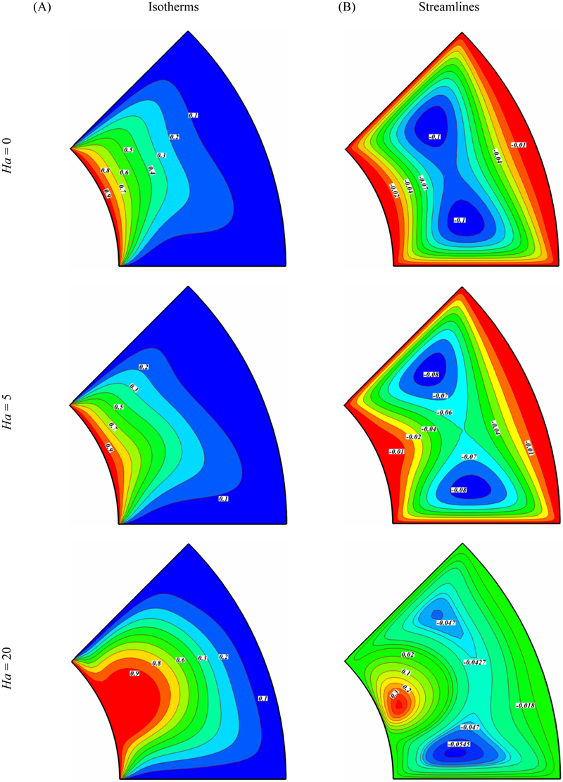
Figure 3.3 (A) Isotherms and (B) streamlines contours for different values of Hartmann number when Re = 10.

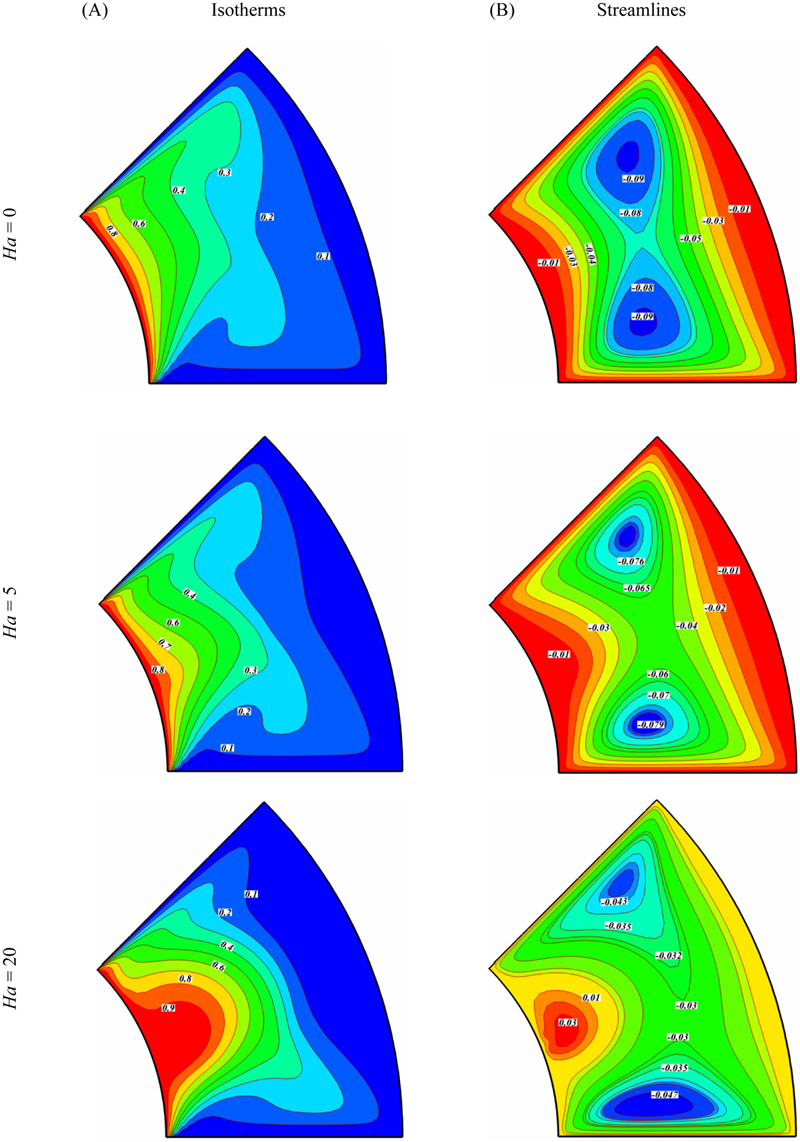
Figure 3.4 (A) Isotherms and (B) streamlines contours for different values of Hartmann number when Re = 100.

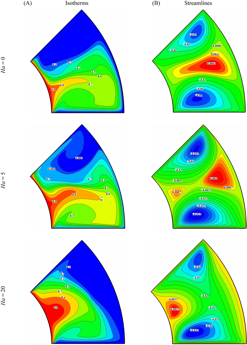
Figure 3.5 (A) Isotherms and (B) streamlines contours for different values of Hartmann number when Re = 1000.

Effects of Hartmann number and Reynolds number on the local and average Nusselt number are shown in Figs. 3.6 and 3.7. Thermal boundary layer thickness increases with a increase in Hartmann number, while it decreases with an augmentation of the Reynolds number. So, Nusselt number increases with an increase in Reynolds number, while it decreases with an increase in Hartmann number. Existence of thermal plumes leads to an extreme local Nusselt number profile.

Figure 3.6 Effects of (A) Reynolds number and (B) Hartmann number on local Nusselt number Nu_loc along hot wall when ɸ = 0.04.

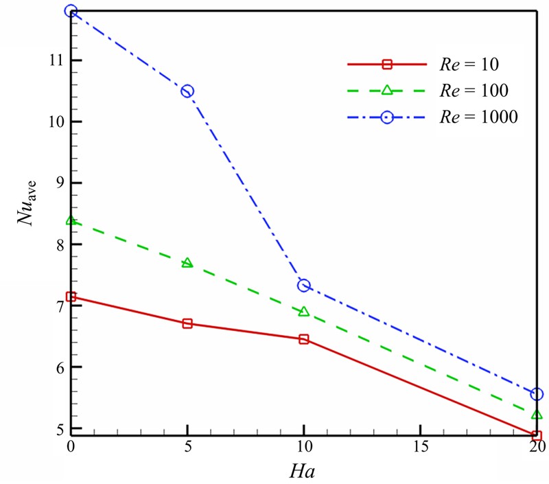
Figure 3.7 Effects of Hartmann number and Reynolds number on local Nusselt number Nu_ave along hot wall when ɸ = 0.04.

Effects of Reynolds number and Hartmann number on the heat transfer enhancement are shown in Fig. 3.8. The effect of nanoparticles is more pronounced at a high Hartmann number than at a low Hartmann number because of the greater enhancement rate. This is because at a high Hartmann number, the heat transfer is dominant by conduction. Therefore, the addition of high-thermal conductivity nanoparticles will increase the conduction and make the enhancement more effective. The heat transfer enhancement decreases with an increase in Reynolds number.

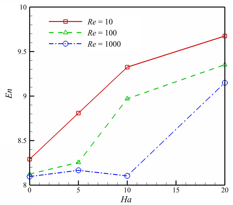
Figure 3.8 Effects of Reynolds number and Hartmann number on heat transfer enhancement.

3.2. MHD nanofluid flow and heat transfer considering viscous dissipation

3.2.1. Problem definition and mathematical model

3.2.1.1. Problem definition

Consider steady flow of nanofluid between two horizontal parallel plates when the fluid and the plates rotate together with a constant angular velocity Ω around the axis that is normal to the plates [3]. A Cartesian coordinate system (x,y,z) is considered as follows: the x-axis is along the plate, the y-axis is perpendicular to it, and the z-axis is normal to the x–y plane (Fig. 3.9). The origin is located at the lower plate, and the plates are located at y = 0 and y = h. The lower plate is stretched by two equal opposite forces, so that the position of the point (0,0,0) remains unchanged. A uniform magnetic flux with density B₀ acts along the y-axis.

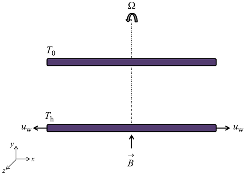
Figure 3.9 The schematic theme of the problem geometry.

Under these assumptions, the Navier–Stokes and energy equations are:

$\frac{\partial u}{\partial x} + \frac{\partial v}{\partial y} + \frac{\partial w}{\partial z} = 0$ $\frac{\partial u}{\partial x} + \frac{\partial v}{\partial y} + \frac{\partial w}{\partial z} = 0$

(3.24)

$ρ_{nf} (u \frac{\partial u}{\partial x} + ν \frac{\partial u}{\partial y} + 2 Ω w) = - \frac{\partial p^{*}}{\partial x} + μ_{nf} (\frac{\partial^{2} u}{\partial x^{2}} + \frac{\partial^{2} u}{\partial y^{2}}) - σ_{nf} B_{0}^{2} u,$ $ρ_{nf} (u \frac{\partial u}{\partial x} + ν \frac{\partial u}{\partial y} + 2 Ω w) = - \frac{\partial p^{*}}{\partial x} + μ_{nf} (\frac{\partial^{2} u}{\partial x^{2}} + \frac{\partial^{2} u}{\partial y^{2}}) - σ_{nf} B_{0}^{2} u,$

(3.25)

$ρ_{nf} (u \frac{\partial v}{\partial y}) = - \frac{\partial p^{*}}{\partial y} + μ_{nf} (\frac{\partial^{2} v}{\partial x^{2}} + \frac{\partial^{2} v}{\partial y^{2}})$ $ρ_{nf} (u \frac{\partial v}{\partial y}) = - \frac{\partial p^{*}}{\partial y} + μ_{nf} (\frac{\partial^{2} v}{\partial x^{2}} + \frac{\partial^{2} v}{\partial y^{2}})$

(3.26)

$ρ_{nf} (u \frac{\partial w}{\partial x} + ν \frac{\partial w}{\partial y} - 2 Ω u) = μ_{nf} (\frac{\partial^{2} w}{\partial x^{2}} + \frac{\partial^{2} w}{\partial y^{2}}) - σ_{nf} B_{0}^{2} w,$ $ρ_{nf} (u \frac{\partial w}{\partial x} + ν \frac{\partial w}{\partial y} - 2 Ω u) = μ_{nf} (\frac{\partial^{2} w}{\partial x^{2}} + \frac{\partial^{2} w}{\partial y^{2}}) - σ_{nf} B_{0}^{2} w,$

(3.27)

$\begin{array}{l} {(ρ C_{p})}_{nf} (u \frac{\partial T}{\partial x} + v \frac{\partial T}{\partial y} + w \frac{\partial T}{\partial z}) = k_{nf} (\frac{\partial^{2} T}{\partial x^{2}} + \frac{\partial^{2} T}{\partial y^{2}} + \frac{\partial^{2} T}{\partial z^{2}}) \\ + μ_{nf} (2 [{(\frac{\partial u}{\partial x})}^{2} + {(\frac{\partial v}{\partial y})}^{2} + {(\frac{\partial w}{\partial z})}^{2}] + {(\frac{\partial v}{\partial x})}^{2} + {(\frac{\partial v}{\partial z})}^{2} + {(\frac{\partial w}{\partial x} + \frac{\partial u}{\partial z})}^{2}) \end{array}$ $\begin{array}{l} {(ρ C_{p})}_{nf} (u \frac{\partial T}{\partial x} + v \frac{\partial T}{\partial y} + w \frac{\partial T}{\partial z}) = k_{nf} (\frac{\partial^{2} T}{\partial x^{2}} + \frac{\partial^{2} T}{\partial y^{2}} + \frac{\partial^{2} T}{\partial z^{2}}) \\ + μ_{nf} (2 [{(\frac{\partial u}{\partial x})}^{2} + {(\frac{\partial v}{\partial y})}^{2} + {(\frac{\partial w}{\partial z})}^{2}] + {(\frac{\partial v}{\partial x})}^{2} + {(\frac{\partial v}{\partial z})}^{2} + {(\frac{\partial w}{\partial x} + \frac{\partial u}{\partial z})}^{2}) \end{array}$

(3.28)

where u,

v

$v$

, and

w

$w$

denote the fluid velocity components along the x, y, and z directions respectively, p* is the modified fluid pressure, T is temperature, and the physical meanings of the other quantities are mentioned in the nomenclature. The absence of ∂p*/∂z in Eq. (3.27) implies that there is a net crossflow along the z-axis. The corresponding boundary conditions are:

$\begin{array}{l} u = a x, v = 0, w = 0, T = T_{h} a t y = 0 \\ u = 0, v = 0, w = 0, T = T_{o} a t y = h \end{array}$ $\begin{array}{l} u = a x, v = 0, w = 0, T = T_{h} a t y = 0 \\ u = 0, v = 0, w = 0, T = T_{o} a t y = h \end{array}$

(3.29)

The effective density, effective heat capacity, and electrical conductivity of the nanofluid are defined as:

$\begin{array}{l} ρ_{nf} = (1 - φ) ρ_{f} + φ ρ_{p}, \\ {(ρ C_{p})}_{nf} = (1 - φ) {(ρ C_{p})}_{f} + φ {(ρ C_{p})}_{p}, \\ \frac{σ_{nf}}{σ_{f}} = 1 + \frac{3 (\frac{σ_{s}}{σ_{f}} - 1) φ}{(\frac{σ_{s}}{σ_{f}} + 2) - (\frac{σ_{s}}{σ_{f}} - 1) φ} . \end{array}$ $\begin{array}{l} ρ_{nf} = (1 - φ) ρ_{f} + φ ρ_{p}, \\ {(ρ C_{p})}_{nf} = (1 - φ) {(ρ C_{p})}_{f} + φ {(ρ C_{p})}_{p}, \\ \frac{σ_{nf}}{σ_{f}} = 1 + \frac{3 (\frac{σ_{s}}{σ_{f}} - 1) φ}{(\frac{σ_{s}}{σ_{f}} + 2) - (\frac{σ_{s}}{σ_{f}} - 1) φ} . \end{array}$

(3.30)

(k_nf) and (μ_nf) are obtained according to the Koo–Kleinstreuer–Li (KKL) model [4]:

$\begin{array}{l} k_{nf} = 1 + \frac{3 (\frac{k_{p}}{k_{f}} - 1) φ}{(\frac{k_{p}}{k_{f}} + 2) - (\frac{k_{p}}{k_{f}} - 1) φ} + 5 \times 10^{4} g^{'} (φ, T, d_{p}) φ ρ_{f} c_{p,f} \sqrt{\frac{κ_{b} T}{ρ_{p} d_{p}}} \\ g^{'} (φ, T, d_{p}) = (a_{6} + a_{7} \ln (d_{p}) + a_{8} \ln (φ) + a_{9} \ln (φ) \ln (d_{p}) + a_{10} \ln {(d_{p})}^{2}) \\ + \ln (T) (a_{1} + a_{2} \ln (d_{p}) + a_{3} \ln (φ) + a_{4} \ln (φ) \ln (d_{p}) + a_{5} \ln {(d_{p})}^{2}) \\ R_{f} + d_{p} / k_{p} = d_{p} / k_{p,eff}, R_{f} = 4 \times 10^{- 8} K m^{2} /W \end{array}$ $\begin{array}{l} k_{nf} = 1 + \frac{3 (\frac{k_{p}}{k_{f}} - 1) φ}{(\frac{k_{p}}{k_{f}} + 2) - (\frac{k_{p}}{k_{f}} - 1) φ} + 5 \times 10^{4} g^{'} (φ, T, d_{p}) φ ρ_{f} c_{p,f} \sqrt{\frac{κ_{b} T}{ρ_{p} d_{p}}} \\ g^{'} (φ, T, d_{p}) = (a_{6} + a_{7} \ln (d_{p}) + a_{8} \ln (φ) + a_{9} \ln (φ) \ln (d_{p}) + a_{10} \ln {(d_{p})}^{2}) \\ + \ln (T) (a_{1} + a_{2} \ln (d_{p}) + a_{3} \ln (φ) + a_{4} \ln (φ) \ln (d_{p}) + a_{5} \ln {(d_{p})}^{2}) \\ R_{f} + d_{p} / k_{p} = d_{p} / k_{p,eff}, R_{f} = 4 \times 10^{- 8} K m^{2} /W \end{array}$

(3.31)

$μ_{nf} = \frac{μ_{f}}{{(1 - φ)}^{2.5}} + \frac{k_{Brownian}}{k_{f}} \times \frac{μ_{f}}{P r}$ $μ_{nf} = \frac{μ_{f}}{{(1 - φ)}^{2.5}} + \frac{k_{Brownian}}{k_{f}} \times \frac{μ_{f}}{P r}$

(3.32)

All needed coefficients and properties are illustrated in Tables 3.2 and 3.3 [4].

Table 3.2

Thermophysical properties of water and nanoparticles [4]

	ρ (kg/m³)	C_p (J/kg·K)	k (W/m·K)	d_p (nm)	σ (Ω·m)⁻¹
Pure water	997.1	4,179	0.613	—	0.05
Al₂O₃	3,970	765	25	47	10⁻¹²
CuO	6,500	540	18	29	10⁻¹⁰

Table 3.3

The coefficient values of Al₂O₃–water nanofluid and CuO-water nanofluid [4]

Coefficient values	Al₂O₃–water	CuO–water
a₁	52.813488759	−26.593310846
a₂	6.115637295	−0.403818333
a₃	0.6955745084	−33.3516805
a₄	4.17455552E-02	−1.915825591
a₅	0.176919300241	6.42185E-02
a₆	−298.19819084	48.40336955
a₇	−34.532716906	−9.787756683
a₈	−3.9225289283	190.245610009
a₉	−0.2354329626	10.9285386565
a₁₀	−0.999063481	−0.72009983664

The following nondimensional variables are introduced:

$\begin{array}{l} η = \frac{y}{h}, u = a x f^{'} (η), ν = - a h f (η), w = a x g (η) \\ θ (η) = \frac{T - T_{o}}{T_{h} - T_{o}} \end{array}$ $\begin{array}{l} η = \frac{y}{h}, u = a x f^{'} (η), ν = - a h f (η), w = a x g (η) \\ θ (η) = \frac{T - T_{o}}{T_{h} - T_{o}} \end{array}$

(3.33)

where the prime denotes differentiation with respect to η.

Therefore, the governing momentum and energy equations for this problem are given in dimensionless form by:

$f^{i v} - R e \frac{A_{1}}{A_{2}} (f^{'} f^{″} - f f^{‴}) - 2 K r \frac{A_{1}}{A_{2}} g^{'} - A_{5} \frac{M}{A_{2}} f^{″} = 0$ $f^{i v} - R e \frac{A_{1}}{A_{2}} (f^{'} f^{″} - f f^{‴}) - 2 K r \frac{A_{1}}{A_{2}} g^{'} - A_{5} \frac{M}{A_{2}} f^{″} = 0$

(3.34)

$g^{″} - R e \frac{A_{1}}{A_{2}} (f^{'} g - f g^{'}) + 2 K r \frac{A_{1}}{A_{2}} f^{'} - A_{5} \frac{M}{A_{2}} g = 0$ $g^{″} - R e \frac{A_{1}}{A_{2}} (f^{'} g - f g^{'}) + 2 K r \frac{A_{1}}{A_{2}} f^{'} - A_{5} \frac{M}{A_{2}} g = 0$

(3.35)

$θ^{″} + P r \frac{A_{2} A_{3}}{A_{1} A_{4}} [R \frac{A_{1}}{A_{2}} f θ^{'} + E c \frac{A_{1}}{A_{3}} (4 {f^{'}}^{2} + g^{2})] = 0$ $θ^{″} + P r \frac{A_{2} A_{3}}{A_{1} A_{4}} [R \frac{A_{1}}{A_{2}} f θ^{'} + E c \frac{A_{1}}{A_{3}} (4 {f^{'}}^{2} + g^{2})] = 0$

(3.36)

The dimensionless quantities in these equations are:

$\begin{array}{l} R e = \frac{a h^{2}}{υ_{f}}, M = \frac{σ_{f} B_{0}^{2} h^{2}}{ρ_{f} υ_{f}}, K r = \frac{Ω h^{2}}{υ_{f}}, P r = \frac{μ_{f} {(ρ C_{p})}_{f}}{ρ_{f} k_{f}}, \\ E c = \frac{ρ_{f} a^{2} h^{2}}{{(ρ C_{p})}_{f} (θ_{0} - θ_{h})}, \\ A_{1} = \frac{ρ_{nf}}{ρ_{f}}, A_{2} = \frac{μ_{nf}}{μ_{f}}, A_{3} = \frac{{(ρ C_{p})}_{nf}}{{(ρ C_{p})}_{f}}, A_{4} = \frac{k_{nf}}{k_{f}}, A_{5} = \frac{σ_{nf}}{σ_{f}} \end{array}$ $\begin{array}{l} R e = \frac{a h^{2}}{υ_{f}}, M = \frac{σ_{f} B_{0}^{2} h^{2}}{ρ_{f} υ_{f}}, K r = \frac{Ω h^{2}}{υ_{f}}, P r = \frac{μ_{f} {(ρ C_{p})}_{f}}{ρ_{f} k_{f}}, \\ E c = \frac{ρ_{f} a^{2} h^{2}}{{(ρ C_{p})}_{f} (θ_{0} - θ_{h})}, \\ A_{1} = \frac{ρ_{nf}}{ρ_{f}}, A_{2} = \frac{μ_{nf}}{μ_{f}}, A_{3} = \frac{{(ρ C_{p})}_{nf}}{{(ρ C_{p})}_{f}}, A_{4} = \frac{k_{nf}}{k_{f}}, A_{5} = \frac{σ_{nf}}{σ_{f}} \end{array}$

(3.37)

Reynolds number (Re) is defined as the ratio of inertial forces to viscous forces and consequently quantifies the relative importance of these two types of forces for given flow conditions. Magnetic parameter (M) is ratio of electromagnetic (Lorentz) force to the viscous force. Rotation parameter (Kr) is ratio of Coriolis force to the viscous force. Prandtl number (Pr) is defined as the ratio of momentum diffusivity (kinematic viscosity) to thermal diffusivity. Eckert number (Ec) expresses the relationship between a flow’s kinetic energy and enthalpy.

The boundary conditions are:

$\begin{array}{l} f = 0, f^{'} = 1, g = 0, θ = 1 & at η = 0 \\ f = 0, f^{'} = 0, g = 0, θ = 0 & at η = 1. \end{array}$ $\begin{array}{l} f = 0, f^{'} = 1, g = 0, θ = 1 & at η = 0 \\ f = 0, f^{'} = 0, g = 0, θ = 0 & at η = 1. \end{array}$

(3.38)

The physical quantity of interest in this problem is the skin friction coefficient C_f along the stretching wall, which is defined as:

$C_{f} = |\frac{A_{2}}{A_{1}} f^{″} (0)| .$ $C_{f} = |\frac{A_{2}}{A_{1}} f^{″} (0)| .$

(3.39)

The Nusselt number at the lower plate is defined as

$N u = |(\frac{k_{nf}}{k_{f}}) θ^{'} (0)|$ $N u = |(\frac{k_{nf}}{k_{f}}) θ^{'} (0)|$

(3.40)

3.2.1.2. Numerical method

Before employing the Runge–Kutta integration scheme, first we reduce the governing differential equations into a set of first-order ODEs.

Let x₁ = η, x₂ = f, x₃ = f′, x₄ = f″, x₅ =

f^{‴}

$f^{‴}$

, x₆ = g, x₇ = g′, x₈ = θ, and x₉ = θ′. We obtain the following system:

$(\begin{array}{c} x_{1}' \\ x_{2}' \\ x_{3}' \\ x_{4}' \\ x_{5}' \\ x_{6}' \\ x_{7}' \\ x_{8}' \\ x_{9}' \end{array}) = (\begin{matrix} 1 \\ x_{3} \\ x_{4} \\ x_{5} \\ R \frac{A_{1}}{A_{2}} (x_{3} x_{4} - x_{2} x_{5}) + 2 K r \frac{A_{1}}{A_{2}} x_{7} + A_{5} \frac{M}{A_{2}} x_{4} \\ x_{7} \\ R \frac{A_{1}}{A_{2}} (x_{3} x_{6} - x_{7} x_{2}) - 2 K r \frac{A_{1}}{A_{2}} x_{3} + A_{5} \frac{M}{A_{2}} x_{6} \\ x_{9} \\ - \Pr \frac{A_{2} A_{3}}{A_{1} A_{4}} [R \frac{A_{1}}{A_{2}} x_{9} x_{2} + E c \frac{A_{1}}{A_{3}} (4 x_{3}^{2} + x_{6}^{2})] \end{matrix})$ $(\begin{array}{c} x_{1}' \\ x_{2}' \\ x_{3}' \\ x_{4}' \\ x_{5}' \\ x_{6}' \\ x_{7}' \\ x_{8}' \\ x_{9}' \end{array}) = (\begin{matrix} 1 \\ x_{3} \\ x_{4} \\ x_{5} \\ R \frac{A_{1}}{A_{2}} (x_{3} x_{4} - x_{2} x_{5}) + 2 K r \frac{A_{1}}{A_{2}} x_{7} + A_{5} \frac{M}{A_{2}} x_{4} \\ x_{7} \\ R \frac{A_{1}}{A_{2}} (x_{3} x_{6} - x_{7} x_{2}) - 2 K r \frac{A_{1}}{A_{2}} x_{3} + A_{5} \frac{M}{A_{2}} x_{6} \\ x_{9} \\ - \Pr \frac{A_{2} A_{3}}{A_{1} A_{4}} [R \frac{A_{1}}{A_{2}} x_{9} x_{2} + E c \frac{A_{1}}{A_{3}} (4 x_{3}^{2} + x_{6}^{2})] \end{matrix})$

(3.41)

and the corresponding initial conditions are

$(\begin{array}{l} x_{1} \\ x_{2} \\ x_{3} \\ x_{4} \\ x_{5} \\ x_{6} \\ x_{7} \\ x_{8} \\ x_{9} \end{array}) = (\begin{matrix} 0 \\ 1 \\ u_{1} \\ u_{2} \\ 0 \\ u_{3} \\ 1 \\ u_{4} \end{matrix})$ $(\begin{array}{l} x_{1} \\ x_{2} \\ x_{3} \\ x_{4} \\ x_{5} \\ x_{6} \\ x_{7} \\ x_{8} \\ x_{9} \end{array}) = (\begin{matrix} 0 \\ 1 \\ u_{1} \\ u_{2} \\ 0 \\ u_{3} \\ 1 \\ u_{4} \end{matrix})$

(3.42)

These nonlinear coupled ODEs along with initial conditions are solved using fourth-order Runge–Kutta integration technique. Suitable values of the unknown initial conditions u₁, u₂, u₃, and u₄ are approximated through Newton’s method until the boundary conditions at f(1) = 0, f′(1) = 0, g(1) =0, and θ(1) = 0 are satisfied. The computations have been performed using MAPLE. The maximum value of x = 1, to each group of parameters is determined when the values of unknown boundary conditions at x = 0 do not change to a successful loop with an error less than 10⁻⁶.

3.2.2. Effects of active parameters

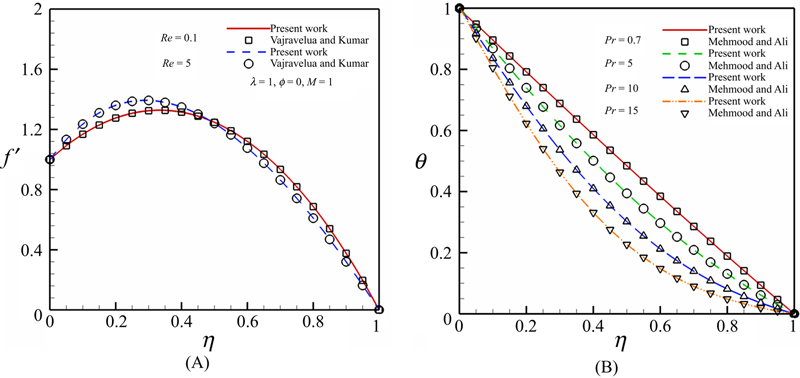
In this study the fourth-order Runge–Kutta method is applied to solve the problem of nanofluid flow and heat transfer characteristics between two horizontal parallel plates in a rotating system. To verify the accuracy of the present results, we have compared the results for the temperature profiles with those reported by Vajravelu and Kumar [5] and Mehmood and Ali [6]. These comparisons show an excellent agreement (Fig. 3.10).

Figure 3.10 Comparison of the velocity and temperature profiles between the present work and (A) Ref. [5]; (B) Ref. [6] for different values of Pr when λ = 0.5, M = 1, Re = 0.5, and Kr = 0.5.

Effect of different kinds of nanoparticles on velocity and temperature profiles is shown in Fig. 3.11. The skin friction coefficient and Nusselt number for different kinds of nanoparticles are shown in Tables 3.4 and 3.5. The skin friction coefficient and Nusselt number change according to different types of nanofluids. This means that the type of nanofluid has a large effect on the cooling and heating processes. Rotation velocity for CuO-water is lower than Al₂O₃-water. An opposite trend is observed for the temperature profile. By selecting CuO as the nanoparticle, a higher Nusselt number and smaller skin friction coefficient is obtained. We choose CuO to assess the effects of active parameters. The effect of Brownian motion on the effective thermal conductivity is considered in the KKL model. This effect can be seen in Fig. 3.12. By considering Brownian motion, a higher effective thermal conductivity and viscosity can be obtained.

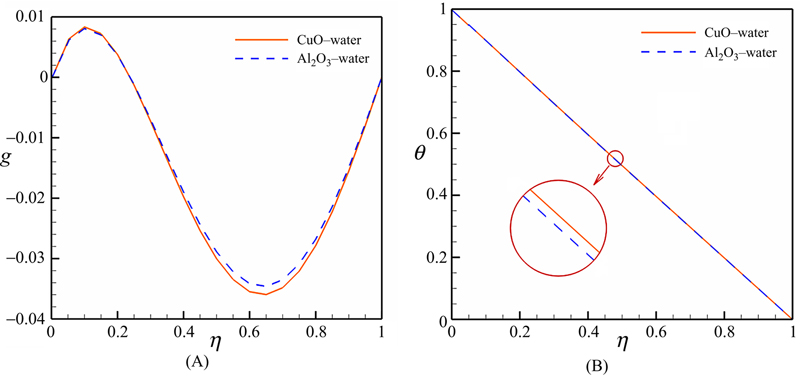
Figure 3.11 (A) Velocity and (B) temperature profiles for different kinds of nanoparticles when M = 1, Kr = 1, Re = 0.1, Ec = 0.01, and ɸ = 0.04.

Table 3.4

Skin friction coefficient for different kinds of nanoparticles when Re = 1 and Kr = 1

M	ɸ = 0.02		ɸ = 0.04
M	CuO	Al₂O₃	CuO	Al₂O₃
0	4.06924	4.095893	3.967395	4.104578
3	4.401786	4.443978	4.261476	4.425107
6	4.714686	4.770744	4.539688	4.727475
9	5.010524	5.079097	4.803935	5.013975

Table 3.5

Nusselt number for different kinds of nanoparticles when Re = 1, Kr = 1, and Ec = 0.01

M	ɸ = 0.02		ɸ = 0.04
M	CuO	Al₂O₃	CuO	Al₂O₃
0	1.425975	1.338769	1.477425	1.363554
3	1.414591	1.326789	1.467274	1.352719
6	1.404375	1.316085	1.458071	1.342948
9	1.395146	1.306454	1.449683	1.334085

Figure 3.12 Effect of Brownian motion on effective (A) thermal conductivity and (B) viscosity.

The effect of the magnetic parameter on the velocity and temperature profiles is shown in Fig. 3.13. Rotational velocity increases with increasing magnetic parameter. Thus the presence of the magnetic field decreases the momentum boundary layer thickness due to Lorenz force. Thermal boundary layer thickness increases with increasing magnetic parameter. Also this figure shows that f decreases with an increase in magnetic parameter and f′ decreases near the bottom wall.

Figure 3.13 Effect of magnetic parameter on (A–C) velocity and (D) temperature profiles when Kr = 1, Re = 0.1, Ec = 0.01, and ɸ = 0.04 (CuO–water).

Fig. 3.14 shows the effects of the magnetic parameter and nanoparticle volume fraction on the skin friction coefficient and Nusselt number. The skin friction coefficient has a reverse relationship with nanoparticle volume fraction. Thermal boundary layer thickness decreases with an increase in nanoparticle volume fraction, and in turn Nusselt number increases with an increase in this parameter. Effect of the magnetic parameter on skin friction coefficient and Nusselt number is opposite to that of the volume fraction of nanoparticles.

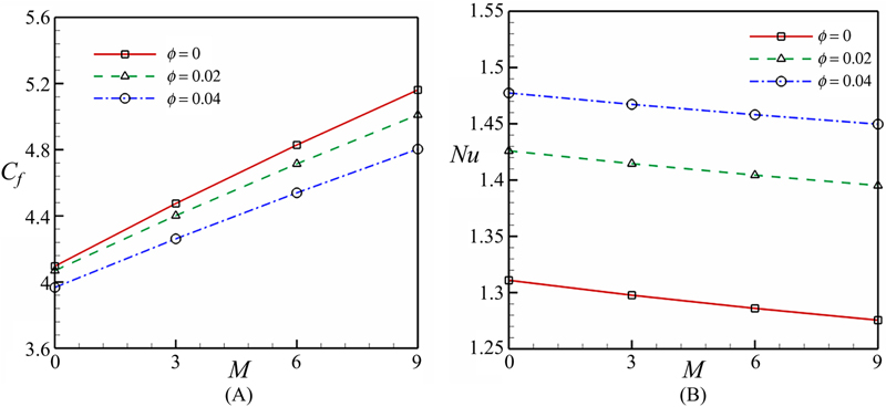
Figure 3.14 Effects of magnetic parameter and nanoparticle volume fraction on (A) skin friction coefficient and (B) Nusselt number when Kr = 1 and Re = 1, and Ec = 0.01 (CuO–water).

Effects of the Reynolds number on velocity, temperature profiles, skin friction coefficient, and Nusselt number are shown in Figs. 3.15 and 3.16. It is worth mentioning that the Reynolds number indicates the relative significance of the inertia effect compared to the viscous effect. Thus, both velocity and temperature profiles decrease as Re increases, and in turn increasing the Reynolds number leads to an increase in the magnitude of the skin friction coefficient and Nusselt number.

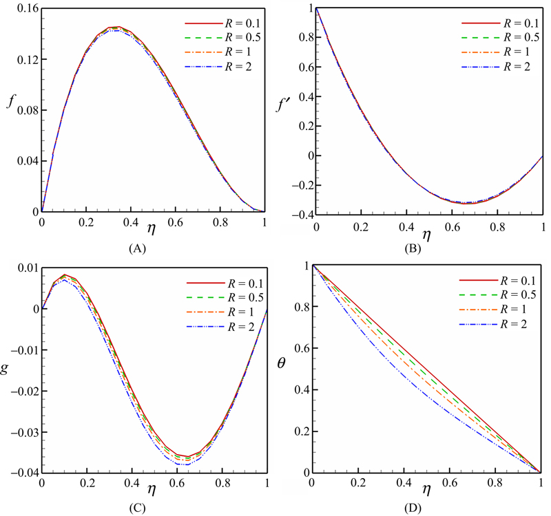
Figure 3.15 Effect of Reynolds number on (A–C) velocity and (D) temperature profiles when M = 1, Kr = 1, Ec = 0.01, and ɸ = 0.04 (CuO–water).

Figure 3.16 Effects of Reynolds number and magnetic parameter on (A) skin friction coefficient and (B) Nusselt number when Kr = 1, ɸ = 0.04, and Ec = 0.01 (CuO–water).

Effects of the rotation parameter on velocity and temperature profiles, skin friction coefficient, and Nusselt number are depicted in Figs. 3.17 and 3.18. As the rotation parameter increases, the Coriolis force increases which results in an increase in both the rotational velocity and temperature profiles. Also increasing the rotation parameter leads to a decrease in the Nusselt number. The skin friction coefficient increases as the rotation parameter increases. Effect of the Eckert number on the temperature profile and Nusselt number is shown in Fig. 3.19. Temperature increases with an increase in viscous dissipation. Nusselt number decreases with an increase in Eckert number.

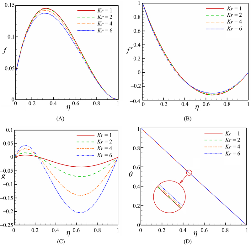
Figure 3.17 Effect of rotation parameter on (A–C) velocity and (D) temperature profiles when M = 1, Re = 0.1, Ec = 0.01, and ɸ = 0.04 (CuO–water).

Figure 3.18 Effects of rotation parameter and magnetic parameter on (A) skin friction coefficient and (B) Nusselt number when Re = 1, ɸ = 0.04, and Ec = 0.01 (CuO–water).

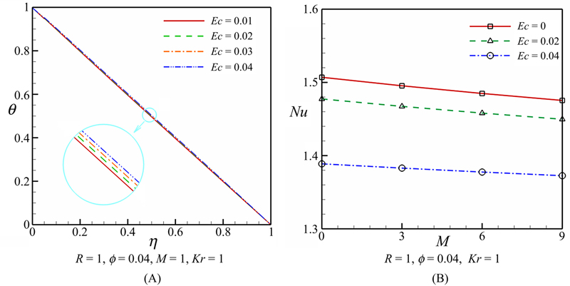
Figure 3.19 Effects of Eckert number on (A) temperature profile and (B) Nusselt number for CuO–water.

3.3. Forced convection heat transfer in a semiannulus under the influence of a variable magnetic field

3.3.1. Problem definition

The physical model along with the needed geometrical parameters and the mesh of the enclosure used in the present CVFEM program are shown in Fig. 3.20 [7]. The outer wall is maintained at constant temperature T_h and the other walls are maintained at a constant temperature T_c. The shape of the inner cylinder profile is assumed to mimic the following form:

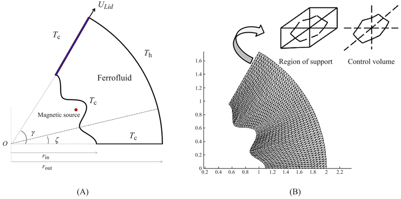
Figure 3.20 (A) Geometry and the boundary conditions and (B) the mesh of enclosure considered in this work.

$r = r_{in} + A \cos (N (ζ)),$ $r = r_{in} + A \cos (N (ζ)),$

(3.43)

in which r_in is the base circle radius, r_out is the radius of the outer cylinder, A and N are amplitude and the number of undulations, respectively, and ζ is the rotation angle. In this study, A and N equal to 0.2 and 4, respectively. For the expression of the magnetic field strength it can be considered that the magnetic source represents a magnetic wire placed vertically to the xy plane at the point

(\bar{a}, \bar{b})

$(\bar{a}, \bar{b})$

. The contours of the magnetic field strength are shown in Fig. 3.21. In this study, the magnetic source is located at (−0.05 cols, 0.5 rows).

Figure 3.21 Contours of the (A) magnetic field strength H, (B) magnetic field intensity component in x direction Hx, and (C) magnetic field intensity component in y direction, Hy.

The flow is steady, two dimensional, laminar, and incompressible. The magnetic Reynolds number is assumed to be small so that the induced magnetic field can be neglected compared to the applied magnetic field. Using the Boussinesq approximation, the governing equations of heat transfer and fluid flow for nanofluid can be obtained as follows:

$\frac{\partial u}{\partial x} + \frac{\partial v}{\partial y} = 0,$ $\frac{\partial u}{\partial x} + \frac{\partial v}{\partial y} = 0,$

(3.44)

$ρ_{nf} (u \frac{\partial u}{\partial x} + v \frac{\partial u}{\partial y}) = - \frac{\partial p}{\partial x} + μ_{nf} (\frac{\partial^{2} u}{\partial x^{2}} + \frac{\partial^{2} u}{\partial y^{2}}) + μ_{0} M \frac{\partial \bar{H}}{\partial x} - σ_{nf} B_{y}^{2} u + σ_{nf} B_{x} B_{y} v,$ $ρ_{nf} (u \frac{\partial u}{\partial x} + v \frac{\partial u}{\partial y}) = - \frac{\partial p}{\partial x} + μ_{nf} (\frac{\partial^{2} u}{\partial x^{2}} + \frac{\partial^{2} u}{\partial y^{2}}) + μ_{0} M \frac{\partial \bar{H}}{\partial x} - σ_{nf} B_{y}^{2} u + σ_{nf} B_{x} B_{y} v,$

(3.45)

$ρ_{nf} (u \frac{\partial v}{\partial x} + v \frac{\partial v}{\partial y}) = - \frac{\partial p}{\partial y} + μ_{nf} (\frac{\partial^{2} v}{\partial x^{2}} + \frac{\partial^{2} v}{\partial y^{2}}) + μ_{0} M \frac{\partial \bar{H}}{\partial y} - σ_{nf} B_{x}^{2} v + σ_{nf} B_{x} B_{y} u,$ $ρ_{nf} (u \frac{\partial v}{\partial x} + v \frac{\partial v}{\partial y}) = - \frac{\partial p}{\partial y} + μ_{nf} (\frac{\partial^{2} v}{\partial x^{2}} + \frac{\partial^{2} v}{\partial y^{2}}) + μ_{0} M \frac{\partial \bar{H}}{\partial y} - σ_{nf} B_{x}^{2} v + σ_{nf} B_{x} B_{y} u,$

(3.46)

$\begin{array}{l} {(ρ C_{p})}_{nf} (u \frac{\partial T}{\partial x} + v \frac{\partial T}{\partial y}) = k_{nf} (\frac{\partial^{2} T}{\partial x^{2}} + \frac{\partial^{2} T}{\partial y^{2}}) + σ_{nf} {(u B_{y} - v B_{x})}^{2} \\ - μ_{0} T \frac{\partial M}{\partial T} (u \frac{\partial \bar{H}}{\partial x} + v \frac{\partial \bar{H}}{\partial y}) + μ_{nf} \{2 {(\frac{\partial u}{\partial x})}^{2} + 2 {(\frac{\partial v}{\partial y})}^{2} + {(\frac{\partial u}{\partial y} + \frac{\partial v}{\partial x})}^{2}\} . \end{array}$ $\begin{array}{l} {(ρ C_{p})}_{nf} (u \frac{\partial T}{\partial x} + v \frac{\partial T}{\partial y}) = k_{nf} (\frac{\partial^{2} T}{\partial x^{2}} + \frac{\partial^{2} T}{\partial y^{2}}) + σ_{nf} {(u B_{y} - v B_{x})}^{2} \\ - μ_{0} T \frac{\partial M}{\partial T} (u \frac{\partial \bar{H}}{\partial x} + v \frac{\partial \bar{H}}{\partial y}) + μ_{nf} \{2 {(\frac{\partial u}{\partial x})}^{2} + 2 {(\frac{\partial v}{\partial y})}^{2} + {(\frac{\partial u}{\partial y} + \frac{\partial v}{\partial x})}^{2}\} . \end{array}$

(3.47)

The terms

μ_{0} M \frac{\partial \bar{H}}{\partial x}

$μ_{0} M \frac{\partial \bar{H}}{\partial x}$

and

μ_{0} M \frac{\partial \bar{H}}{\partial y}

$μ_{0} M \frac{\partial \bar{H}}{\partial y}$

in Eqs. (3.46) and (3.47), respectively, represent the components of magnetic force per unit volume, and depend on the existence of the magnetic gradient on the corresponding x and y directions. These two terms are well known from Ferrohydrodynamics (FHD), which is the so-called Kelvin force. The terms

- σ_{nf} B_{y}^{2} u + σ_{nf} B_{x} B_{y} v

$- σ_{nf} B_{y}^{2} u + σ_{nf} B_{x} B_{y} v$

and

- σ_{nf} B_{x}^{2} v + σ_{nf} B_{x} B_{y} u

$- σ_{nf} B_{x}^{2} v + σ_{nf} B_{x} B_{y} u$

appearing in Eqs. (3.45) and (3.46), respectively, represent the Lorentz force per unit volume toward the x and y directions, and arise due to the electrical conductivity of the fluid. These two terms are known in MHD. The principles of MHD and FHD are combined in the mathematical model presented in Ref. [2] and the aforementioned terms arise together in the governing equations Eqs. (3.45) and (3.46). The term

μ_{0} T \frac{\partial M}{\partial T} (u \frac{\partial \bar{H}}{\partial x} + v \frac{\partial \bar{H}}{\partial y})

$μ_{0} T \frac{\partial M}{\partial T} (u \frac{\partial \bar{H}}{\partial x} + v \frac{\partial \bar{H}}{\partial y})$

in Eq. (3.47) represents the thermal power per unit volume due to the magnetocaloric effect. Also the term σ_nf (uB_y − vB_x)² in Eq. (3.47) represents the Joule heating. For the variation of the magnetization M, with the magnetic field intensity

\bar{H}

$\bar{H}$

, and temperature T the following relation derived in Ref. [2] is considered:

$M = K^{'} \bar{H} ({T^{'}}_{c} - T)$ $M = K^{'} \bar{H} ({T^{'}}_{c} - T)$

(3.48)

where K′ is a constant and

{T^{'}}_{c}

${T^{'}}_{c}$

is the Curie temperature.

In these equations, μ₀ is the magnetic permeability of vacuum (4π × 10⁻⁷ Tm/A),

\bar{H}

$\bar{H}$

is the magnetic field strength,

\bar{B}

$\bar{B}$

is the magnetic induction

(\bar{B} = μ_{0} \bar{H})

$(\bar{B} = μ_{0} \bar{H})$

, and the bar above the quantities denotes that they are dimensional. The effective density (ρ_nf) and heat capacitance

{(ρ C_{p})}_{nf}

${(ρ C_{p})}_{nf}$

of the nanofluid are defined as

$ρ_{nf} = ρ_{f} (1 - φ) + ρ_{s} φ,$ $ρ_{nf} = ρ_{f} (1 - φ) + ρ_{s} φ,$

(3.49)

${(ρ C_{p})}_{nf} = {(ρ C_{p})}_{f} (1 - φ) + {(ρ C_{p})}_{s} φ,$ ${(ρ C_{p})}_{nf} = {(ρ C_{p})}_{f} (1 - φ) + {(ρ C_{p})}_{s} φ,$

(3.50)

where ɸ is the solid volume fraction of nanoparticles.

Thermal diffusivity, dynamic viscosity, thermal conductivity, and effective electrical conductivity of the nanofluids is

$α_{nf} = \frac{k_{nf}}{{(ρ C_{p})}_{nf}},$ $α_{nf} = \frac{k_{nf}}{{(ρ C_{p})}_{nf}},$

(3.51)

$μ_{nf} = \frac{μ_{f}}{{(1 - φ)}^{2.5}} .$ $μ_{nf} = \frac{μ_{f}}{{(1 - φ)}^{2.5}} .$

(3.52)

$\frac{k_{nf}}{k_{f}} = \frac{k_{s} + 2 k_{f} - 2 φ (k_{f} - k_{s})}{k_{s} + 2 k_{f} + φ (k_{f} - k_{s})},$ $\frac{k_{nf}}{k_{f}} = \frac{k_{s} + 2 k_{f} - 2 φ (k_{f} - k_{s})}{k_{s} + 2 k_{f} + φ (k_{f} - k_{s})},$

(3.53)

$\frac{σ_{nf}}{σ_{f}} = 1 + \frac{3 (\frac{σ_{s}}{σ_{f}} - 1) φ}{(\frac{σ_{s}}{σ_{f}} + 2) - (\frac{σ_{s}}{σ_{f}} - 1) φ} .$ $\frac{σ_{nf}}{σ_{f}} = 1 + \frac{3 (\frac{σ_{s}}{σ_{f}} - 1) φ}{(\frac{σ_{s}}{σ_{f}} + 2) - (\frac{σ_{s}}{σ_{f}} - 1) φ} .$

(3.54)

By introducing the following nondimensional variables:

$\begin{array}{l} a = \frac{\bar{a}}{L}, b = \frac{\bar{b}}{L}, X = \frac{x}{L}, Y = \frac{y}{L}, Θ = \frac{T - T_{c}}{T_{h} - T_{c}}, U = \frac{u}{u_{r}}, V = \frac{v}{u_{r}}, \\ H = \frac{\bar{H}}{\bar{H_{0}}}, H_{x} = \frac{\bar{H_{x}}}{\bar{H_{0}}}, H_{y} = \frac{\bar{H_{y}}}{\bar{H_{0}}}, P = \frac{p}{ρ_{f} {(u_{r})}^{2}}, \end{array}$ $\begin{array}{l} a = \frac{\bar{a}}{L}, b = \frac{\bar{b}}{L}, X = \frac{x}{L}, Y = \frac{y}{L}, Θ = \frac{T - T_{c}}{T_{h} - T_{c}}, U = \frac{u}{u_{r}}, V = \frac{v}{u_{r}}, \\ H = \frac{\bar{H}}{\bar{H_{0}}}, H_{x} = \frac{\bar{H_{x}}}{\bar{H_{0}}}, H_{y} = \frac{\bar{H_{y}}}{\bar{H_{0}}}, P = \frac{p}{ρ_{f} {(u_{r})}^{2}}, \end{array}$

(3.55)

where in Eq. (3.55)

\bar{H_{0}} = \bar{H} (\bar{a}, 0) = \frac{γ}{2 π | b |}

$\bar{H_{0}} = \bar{H} (\bar{a}, 0) = \frac{γ}{2 π | b |}$

and L = r_out − r_in; and using them in Eqs. (3.44)–(3.47), we get

$\frac{\partial U}{\partial X} + \frac{\partial V}{\partial Y} = 0,$ $\frac{\partial U}{\partial X} + \frac{\partial V}{\partial Y} = 0,$

(3.56)

$\begin{array}{l} U \frac{\partial U}{\partial X} + V \frac{\partial U}{\partial Y} = - \frac{\partial P}{\partial X} + \frac{1}{R e} [\frac{μ_{nf} / μ_{f}}{ρ_{nf} / ρ_{f}}] (\frac{\partial^{2} U}{\partial X^{2}} + \frac{\partial^{2} U}{\partial Y^{2}}) \\ + M n_{F} (\frac{ρ_{f}}{ρ_{nf}}) (ɛ_{2} - ɛ_{1} - Θ) H \frac{\partial H}{\partial X} - \frac{H a^{2}}{R e} [\frac{σ_{nf} / σ_{f}}{ρ_{nf} / ρ_{f}}] (H_{y}^{2} U - H_{x} H_{y} V), \end{array}$ $\begin{array}{l} U \frac{\partial U}{\partial X} + V \frac{\partial U}{\partial Y} = - \frac{\partial P}{\partial X} + \frac{1}{R e} [\frac{μ_{nf} / μ_{f}}{ρ_{nf} / ρ_{f}}] (\frac{\partial^{2} U}{\partial X^{2}} + \frac{\partial^{2} U}{\partial Y^{2}}) \\ + M n_{F} (\frac{ρ_{f}}{ρ_{nf}}) (ɛ_{2} - ɛ_{1} - Θ) H \frac{\partial H}{\partial X} - \frac{H a^{2}}{R e} [\frac{σ_{nf} / σ_{f}}{ρ_{nf} / ρ_{f}}] (H_{y}^{2} U - H_{x} H_{y} V), \end{array}$

(3.57)

$\begin{array}{l} U \frac{\partial V}{\partial X} + V \frac{\partial V}{\partial Y} = - \frac{\partial P}{\partial X} + \frac{1}{R e} [\frac{μ_{nf} / μ_{f}}{ρ_{nf} / ρ_{f}}] (\frac{\partial^{2} V}{\partial X^{2}} + \frac{\partial^{2} V}{\partial Y^{2}}) \\ + M n_{F} (\frac{ρ_{f}}{ρ_{nf}}) (ɛ_{2} - ɛ_{1} - Θ) H \frac{\partial H}{\partial Y} - \frac{H a^{2}}{R e} [\frac{σ_{nf} / σ_{f}}{ρ_{nf} / ρ_{f}}] (H_{x}^{2} V - H_{x} H_{y} U), \end{array}$ $\begin{array}{l} U \frac{\partial V}{\partial X} + V \frac{\partial V}{\partial Y} = - \frac{\partial P}{\partial X} + \frac{1}{R e} [\frac{μ_{nf} / μ_{f}}{ρ_{nf} / ρ_{f}}] (\frac{\partial^{2} V}{\partial X^{2}} + \frac{\partial^{2} V}{\partial Y^{2}}) \\ + M n_{F} (\frac{ρ_{f}}{ρ_{nf}}) (ɛ_{2} - ɛ_{1} - Θ) H \frac{\partial H}{\partial Y} - \frac{H a^{2}}{R e} [\frac{σ_{nf} / σ_{f}}{ρ_{nf} / ρ_{f}}] (H_{x}^{2} V - H_{x} H_{y} U), \end{array}$

(3.58)

$\begin{array}{l} U \frac{\partial Θ}{\partial X} + V \frac{\partial Θ}{\partial Y} = [\frac{k_{nf} / k_{f}}{{(ρ C_{p})}_{nf} / {(ρ C_{p})}_{f}}] (\frac{\partial^{2} Θ}{\partial X^{2}} + \frac{\partial^{2} Θ}{\partial Y^{2}}) \\ + H a^{2} E c [\frac{σ_{nf} / σ_{f}}{{(ρ C_{p})}_{nf} / {(ρ C_{p})}_{f}}] {\{U H_{y} - V H_{x}\}}^{2} \\ + M n_{F} E c \frac{{(ρ C_{p})}_{f}}{{(ρ C_{p})}_{nf}} \{U \frac{\partial H}{\partial X} + V \frac{\partial H}{\partial Y}\} H (ɛ_{1} + Θ) + E c [\frac{μ_{nf} / μ_{f}}{{(ρ C_{p})}_{nf} / {(ρ C_{p})}_{f}}] \{2 {(\frac{\partial U}{\partial X})}^{2} + 2 {(\frac{\partial V}{\partial Y})}^{2} + {(\frac{\partial U}{\partial Y} + \frac{\partial V}{\partial X})}^{2}\}, \end{array}$ $\begin{array}{l} U \frac{\partial Θ}{\partial X} + V \frac{\partial Θ}{\partial Y} = [\frac{k_{nf} / k_{f}}{{(ρ C_{p})}_{nf} / {(ρ C_{p})}_{f}}] (\frac{\partial^{2} Θ}{\partial X^{2}} + \frac{\partial^{2} Θ}{\partial Y^{2}}) \\ + H a^{2} E c [\frac{σ_{nf} / σ_{f}}{{(ρ C_{p})}_{nf} / {(ρ C_{p})}_{f}}] {\{U H_{y} - V H_{x}\}}^{2} \\ + M n_{F} E c \frac{{(ρ C_{p})}_{f}}{{(ρ C_{p})}_{nf}} \{U \frac{\partial H}{\partial X} + V \frac{\partial H}{\partial Y}\} H (ɛ_{1} + Θ) + E c [\frac{μ_{nf} / μ_{f}}{{(ρ C_{p})}_{nf} / {(ρ C_{p})}_{f}}] \{2 {(\frac{\partial U}{\partial X})}^{2} + 2 {(\frac{\partial V}{\partial Y})}^{2} + {(\frac{\partial U}{\partial Y} + \frac{\partial V}{\partial X})}^{2}\}, \end{array}$

(3.59)

where

R e = \frac{ρ_{f} L u_{r}}{μ_{f}}, H a = L H_{0} μ_{0} \sqrt{σ_{f} / μ_{f}}, ɛ_{1} = T_{1} / ∆ T, ɛ_{2} = {T^{'}}_{c} / ∆ T, E c = (ρ_{f} u_{r}^{2}) / [{(ρ C_{p})}_{f} ∆ T]

$R e = \frac{ρ_{f} L u_{r}}{μ_{f}}, H a = L H_{0} μ_{0} \sqrt{σ_{f} / μ_{f}}, ɛ_{1} = T_{1} / ∆ T, ɛ_{2} = {T^{'}}_{c} / ∆ T, E c = (ρ_{f} u_{r}^{2}) / [{(ρ C_{p})}_{f} ∆ T]$

and

M n_{F} = μ_{0} H_{0}^{2} K^{'} (T_{h} - T_{c}) / (ρ_{f} u_{r}^{2})

$M n_{F} = μ_{0} H_{0}^{2} K^{'} (T_{h} - T_{c}) / (ρ_{f} u_{r}^{2})$

are the Reynolds number, the Hartman number, the temperature number, the Curie temperature number, Eckert number, and the magnetic number arising from FHD the for the base fluid, respectively. The stream function and vorticity are defined as

$\begin{array}{l} u = \frac{\partial ψ}{\partial y}, v = - \frac{\partial ψ}{\partial x}, ω = \frac{\partial v}{\partial x} - \frac{\partial u}{\partial y}, \\ Ω = \frac{ω L}{u_{r}}, Ψ = \frac{ψ}{L u_{r}} . \end{array}$ $\begin{array}{l} u = \frac{\partial ψ}{\partial y}, v = - \frac{\partial ψ}{\partial x}, ω = \frac{\partial v}{\partial x} - \frac{\partial u}{\partial y}, \\ Ω = \frac{ω L}{u_{r}}, Ψ = \frac{ψ}{L u_{r}} . \end{array}$

(3.60)

The stream function satisfies the continuity Eq. (3.56). The vorticity equation is obtained by eliminating the pressure between the two momentum equations. The appropriate boundary conditions can be written as

$\begin{array}{l} Θ = 1.0 & on the outer circular boundary, \\ Θ = 0.0 & other walls boundaries, and \\ Ψ = 0.0 & on all solid boundaries . \end{array}$ $\begin{array}{l} Θ = 1.0 & on the outer circular boundary, \\ Θ = 0.0 & other walls boundaries, and \\ Ψ = 0.0 & on all solid boundaries . \end{array}$

(3.61)

The values of vorticity on the boundary of the enclosure can be obtained using the stream function formulation and the known velocity conditions during the iterative solution procedure.

The local Nusselt number of the nanofluid along the hot wall can be expressed as

$N u_{loc} = (\frac{k_{nf}}{k_{f}}) \frac{\partial Θ}{\partial r},$ $N u_{loc} = (\frac{k_{nf}}{k_{f}}) \frac{\partial Θ}{\partial r},$

(3.62)

where r is the radial direction. The average Nusselt number on the cold circular wall is evaluated as:

$N u_{ave} = \frac{1}{π / 3} \int_{0}^{π / 3} N u_{loc} (ζ) d ζ .$ $N u_{ave} = \frac{1}{π / 3} \int_{0}^{π / 3} N u_{loc} (ζ) d ζ .$

(3.63)

3.3.2. Effects of active parameters

Forced convection heat transfer of ferrofluid in a lid-driven semiannulus enclosure in the presence of external magnetic field is studied using CVFEM. FHD and MHD are combined to obtain a suitable mathematical model. Calculations are made for various values of the volume fraction of the nanoparticles (ɸ = 0 and 4%), the Reynolds number (Re = 10–600), the magnetic number arising from FHD (Mn_F = 0, 2, 6, and 10), and the Hartmann number arising from MHD (Ha = 0, 2, 6, and 10). In all calculations, the Prandtl number (Pr), the temperature number (ɛ₁), and the Eckert number (Ec) are set to 6.8, 0.0, and 10⁻⁵, respectively. Effects of nanoparticles on the isotherms and the streamlines are shown in Fig. 3.22. Thermal boundary layer thickness increases with an increase in the nanofluid volume fraction. Also, velocity increased with the addition of nanoparticles.

Figure 3.22 Comparison of the isotherms and streamlines between (A) nanofluid (ɸ = 0.04) and (B) pure fluid (ɸ = 0) when Mn_F = 10, Ha = 10, Re = 600, and Pr = 6.8.

Effects of the Reynolds number, the Hartmann number, and the magnetic number on isotherms and streamlines are shown in Figs. 3.23 and 3.24. An increase in the Lorentz force leads to an increase in the thermal boundary layer thickness and a reduction in the velocity field. Thermal boundary layer thickness decreases with an increase in the Kelvin forces, and thermal plume appears over the outer layer. As the Reynolds number increases, the absolute value of the stream function increases, and thermal plume is generated due to two strong eddies. The thermal plume disappears as the Hartmann number increases. It is an interesting observation that as the magnetic number increases and when the Reynolds number is large, the main eddies turn into four smaller eddies. Also, it can be seen that the effect of magnetic number on isotherms is more pronounced for higher values of Reynolds number.

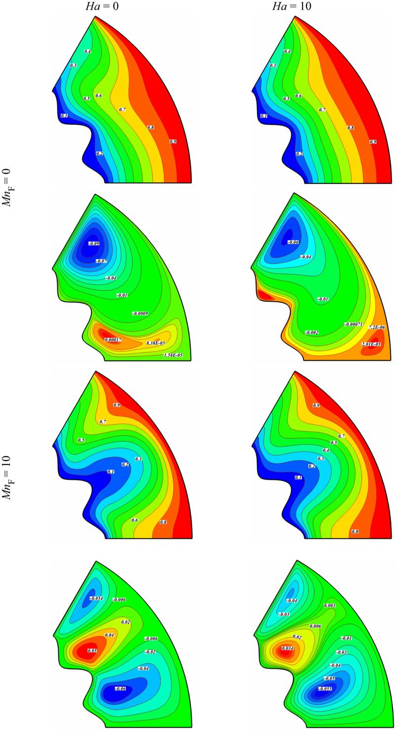
Figure 3.23 Isotherms (up) and streamlines (down) contours for different values of Hartmann number and magnetic number when Re = 10, ɸ = 0.04, and Pr = 6.8.

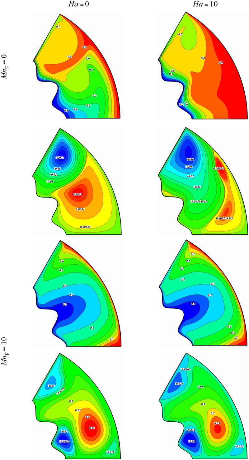
Figure 3.24 Isotherms (up) and streamlines (down) contours for different values of Hartmann number and magnetic number when Re = 600, ɸ = 0.04, and Pr = 6.8.

Effects of the magnetic number, the Hartmann number, and the Reynolds number on the local and the average Nusselt numbers are shown Figs. 3.25 and 3.26, respectively. A local maximum and a minimum in local Nusselt number profile exist due to the existence of a thermal plume. The Nusselt number increases with an increase in the Reynolds number and the magnetic number, but it decreases with the augmentation of the Hartmann number. Effects of the Reynolds number, the Hartmann number, and the magnetic number on heat transfer are shown in Fig. 3.27. Heat transfer enhances with an increase in the Reynolds number and the magnetic number, while the opposite trend is observed with the Hartmann number.

Figure 3.25 (A–D) Effects of magnetic number, Hartmann number, and Reynolds number on local Nusselt number (Nu_loc) along hot wall when ɸ = 0.04.

Figure 3.26 (A–B) Effects of Reynolds number, Hartmann number, and magnetic number on average Nusselt number when ɸ = 0.04.

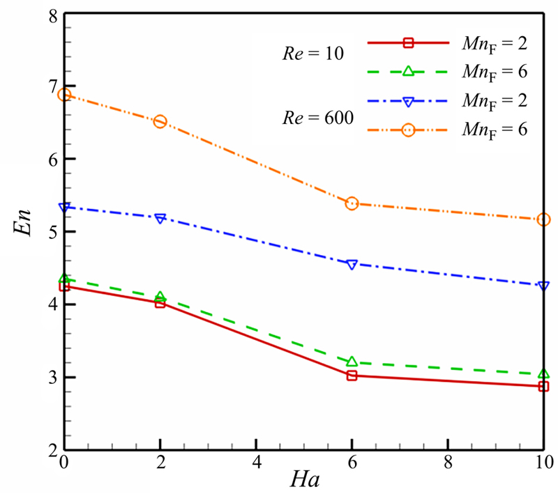
Figure 3.27 Effects of Reynolds number, Hartmann number, and magnetic number on heat transfer enhancement.

3.4. MHD nanofluid flow and heat transfer considering viscous dissipation

3.4.1. Problem definition and mathematical model

3.4.1.1. Problem definition

Consider the steady laminar nanofluid flow caused by a stretching tube with radius a in the axial direction in a fluid (Fig. 3.28), where the z-axis is measured along the axis of the tube and the r-axis is measured in the radial direction [8]. It is assumed that the surface of the tube has constant temperature T_w and the ambient fluid temperature is T_∞ (T_w > T_∞). The viscous dissipation is neglected, as it is assumed to be small. It is assumed that the base fluid and the nanoparticles are in thermal equilibrium and no slip occurs between them. Under these assumptions the governing equations are:

Vector form:

$\vec{\nabla} . \vec{V} = 0$ $\vec{\nabla} . \vec{V} = 0$

(3.64)

$ρ_{nf} (\frac{\partial \vec{V}}{\partial t} + (\vec{V} . \vec{\nabla}) \vec{V}) = - \vec{\nabla} P + μ_{nf} \nabla^{2} \vec{V}$ $ρ_{nf} (\frac{\partial \vec{V}}{\partial t} + (\vec{V} . \vec{\nabla}) \vec{V}) = - \vec{\nabla} P + μ_{nf} \nabla^{2} \vec{V}$

(3.65)

${(ρ C_{p})}_{n f} (\frac{\partial T}{\partial t} + (\vec{V} . \vec{\nabla}) T) = k_{nf} \nabla^{2} T$ ${(ρ C_{p})}_{n f} (\frac{\partial T}{\partial t} + (\vec{V} . \vec{\nabla}) T) = k_{nf} \nabla^{2} T$

(3.66)

where

\vec{V} = (u, v, w)

$\vec{V} = (u, v, w)$

is velocity vector, T is temperature, P is pressure, ρ_nf, μ_nf,

{(ρ C_{p})}_{nf}

${(ρ C_{p})}_{nf}$

, k_nf are density, viscosity, heat capacitance, and thermal conductivity of nanofluid, respectively. Also the operation of

\vec{\nabla}

$\vec{\nabla}$

can be defined as

\vec{\nabla} = (\frac{\partial}{\partial x}, \frac{\partial}{\partial y}, \frac{\partial}{\partial z})

$\vec{\nabla} = (\frac{\partial}{\partial x}, \frac{\partial}{\partial y}, \frac{\partial}{\partial z})$

Scalar form:

$\frac{\partial (r w)}{\partial z} + \frac{\partial (r u)}{\partial r} = 0,$ $\frac{\partial (r w)}{\partial z} + \frac{\partial (r u)}{\partial r} = 0,$

(3.67)

$ρ_{nf} (w \frac{\partial w}{\partial z} + u \frac{\partial w}{\partial r}) = μ_{nf} (\frac{\partial^{2} w}{\partial r^{2}} + \frac{1}{r} \frac{\partial w}{\partial r}),$ $ρ_{nf} (w \frac{\partial w}{\partial z} + u \frac{\partial w}{\partial r}) = μ_{nf} (\frac{\partial^{2} w}{\partial r^{2}} + \frac{1}{r} \frac{\partial w}{\partial r}),$

(3.68)

$ρ_{nf} (w \frac{\partial u}{\partial z} + u \frac{\partial u}{\partial r}) = - \frac{\partial P}{\partial r} + μ_{nf} (\frac{\partial^{2} u}{\partial r^{2}} + \frac{1}{r} \frac{\partial u}{\partial r} - \frac{u}{r^{2}}),$ $ρ_{nf} (w \frac{\partial u}{\partial z} + u \frac{\partial u}{\partial r}) = - \frac{\partial P}{\partial r} + μ_{nf} (\frac{\partial^{2} u}{\partial r^{2}} + \frac{1}{r} \frac{\partial u}{\partial r} - \frac{u}{r^{2}}),$

(3.69)

$(w \frac{\partial T}{\partial z} + u \frac{\partial T}{\partial r}) = \frac{k_{nf}}{{(ρ C_{p})}_{nf}} (\frac{\partial^{2} T}{\partial r^{2}} + \frac{1}{r} \frac{\partial T}{\partial r}),$ $(w \frac{\partial T}{\partial z} + u \frac{\partial T}{\partial r}) = \frac{k_{nf}}{{(ρ C_{p})}_{nf}} (\frac{\partial^{2} T}{\partial r^{2}} + \frac{1}{r} \frac{\partial T}{\partial r}),$

(3.70)

subject to the boundary conditions

$\begin{array}{l} r = a : u = U_{w}, w = w_{w}, T = T_{w} \\ r \to \infty : w \to 0, T \to T_{\infty} \end{array}$ $\begin{array}{l} r = a : u = U_{w}, w = w_{w}, T = T_{w} \\ r \to \infty : w \to 0, T \to T_{\infty} \end{array}$

(3.71)

where

U_{w} = - c a γ, w_{w} = 2 c z

$U_{w} = - c a γ, w_{w} = 2 c z$

and c is a positive constant. γ is a constant in which γ > 0 and γ < 0 corresponding to mass suction and mass injection, respectively.

The effective density (ρ_nf) and the heat capacitance

{(ρ C_{p})}_{nf}

${(ρ C_{p})}_{nf}$

of the nanofluid are given as:

$ρ_{nf} = ρ_{f} (1 - φ) + ρ_{s} φ$ $ρ_{nf} = ρ_{f} (1 - φ) + ρ_{s} φ$

(3.72)

${(ρ C_{p})}_{nf} = {(ρ C_{p})}_{f} (1 - φ) + {(ρ C_{p})}_{s} φ$ ${(ρ C_{p})}_{nf} = {(ρ C_{p})}_{f} (1 - φ) + {(ρ C_{p})}_{s} φ$

(3.73)

Here, ɸ is the solid volume fraction.

(k_nf) and (μ_nf) are obtained according to the KKL model [4]:

(3.74)

$μ_{nf} = \frac{μ_{f}}{{(1 - φ)}^{2.5}} + \frac{k_{Brownian}}{k_{f}} \times \frac{μ_{f}}{P r}$ $μ_{nf} = \frac{μ_{f}}{{(1 - φ)}^{2.5}} + \frac{k_{Brownian}}{k_{f}} \times \frac{μ_{f}}{P r}$

(3.75)

Following Wang [9] we take the similarity transformation:

$η = {(r / a)}^{2}, u = - c a [f (η) / \sqrt{η}], w = 2 c f^{'} (η) z, θ (η) = (T - T_{\infty}) / (T_{w} - T_{\infty}),$ $η = {(r / a)}^{2}, u = - c a [f (η) / \sqrt{η}], w = 2 c f^{'} (η) z, θ (η) = (T - T_{\infty}) / (T_{w} - T_{\infty}),$

(3.76)

where prime denotes differentiation with respect to η.

Substituting Eq. (3.76) in to Eqs. (3.68) and (3.70), we get the following ordinary differential equations:

$Re . \frac{A_{1}}{A_{4}} ({f^{'}}^{2} - f f^{″}) = η f^{‴} + f^{″},$ $Re . \frac{A_{1}}{A_{4}} ({f^{'}}^{2} - f f^{″}) = η f^{‴} + f^{″},$

(3.77)

$η θ^{″} + (1 + R z P r f . A_{2} / A_{3}) θ^{'} = 0,$ $η θ^{″} + (1 + R z P r f . A_{2} / A_{3}) θ^{'} = 0,$

(3.78)

where

R e = c a^{2} / 2 υ_{f}

$R e = c a^{2} / 2 υ_{f}$

is the Reynolds number,

υ_{f} = μ_{f} / ρ_{f}

$υ_{f} = μ_{f} / ρ_{f}$

the kinematic viscosity,

P r = μ_{f} {(ρ C_{p})}_{f} / (ρ_{f} k_{f})

$P r = μ_{f} {(ρ C_{p})}_{f} / (ρ_{f} k_{f})$

is the Prandtl number, and A₁, A₂, A₃, and A₄ are parameters having the following forms:

$A_{1} = (1 - φ) + \frac{ρ_{s}}{ρ_{f}} φ$ $A_{1} = (1 - φ) + \frac{ρ_{s}}{ρ_{f}} φ$

(3.79)

$A_{2} = (1 - φ) + \frac{{(ρ C_{p})}_{s}}{{(ρ C_{p})}_{f}} φ$ $A_{2} = (1 - φ) + \frac{{(ρ C_{p})}_{s}}{{(ρ C_{p})}_{f}} φ$

(3.80)

$A_{3} = \frac{k_{nf}}{k_{f}}, A_{4} = \frac{μ_{nf}}{μ_{f}}$ $A_{3} = \frac{k_{nf}}{k_{f}}, A_{4} = \frac{μ_{nf}}{μ_{f}}$

(3.81)

The boundary conditions (3.71) become

$\begin{array}{l} f (1) = γ, & f^{'} (1) = 1, & θ (1) = 1, \\ f^{'} (\infty) \to 0, & θ (\infty) \to 0. \end{array}$ $\begin{array}{l} f (1) = γ, & f^{'} (1) = 1, & θ (1) = 1, \\ f^{'} (\infty) \to 0, & θ (\infty) \to 0. \end{array}$

(3.82)

The pressure (P) can now be determined from Eq. (3.69) in the form

$\frac{P}{ρ_{nf}} = \frac{P_{\infty}}{ρ_{nf}} - \frac{c^{2} a^{2}}{2 η} f^{2} (η) - 2 c υ_{nf} f^{'} (η),$ $\frac{P}{ρ_{nf}} = \frac{P_{\infty}}{ρ_{nf}} - \frac{c^{2} a^{2}}{2 η} f^{2} (η) - 2 c υ_{nf} f^{'} (η),$

(3.83)

that is,

$\frac{P - P_{\infty}}{ρ_{nf} c υ_{nf}} = - \frac{R e}{η} . \frac{A_{1}}{A_{4}} f^{2} (η) - 2 f^{'} (η) .$ $\frac{P - P_{\infty}}{ρ_{nf} c υ_{nf}} = - \frac{R e}{η} . \frac{A_{1}}{A_{4}} f^{2} (η) - 2 f^{'} (η) .$

(3.84)

Physical quantities of interest are the skin friction coefficient (C_f) and the Nusselt number (Nu), which are defined as

$C_{f} = \frac{τ_{w}}{ρ w_{w}^{2} / 2^{'}} N u = \frac{a q_{w}}{k_{f} (T_{w} - T_{\infty})},$ $C_{f} = \frac{τ_{w}}{ρ w_{w}^{2} / 2^{'}} N u = \frac{a q_{w}}{k_{f} (T_{w} - T_{\infty})},$

(3.85)

with k_f being the thermal conductivity of the base fluid. Further,

τ_{w}

$τ_{w}$

and

q_{w}

$q_{w}$

are the surface shear stress and the surface heat flux, respectively, and they are given by

$τ_{w} = μ_{nf} {(\frac{\partial w}{\partial r})}_{r = a}, q_{w} = - k_{nf} {(\frac{\partial T}{\partial r})}_{r = a},$ $τ_{w} = μ_{nf} {(\frac{\partial w}{\partial r})}_{r = a}, q_{w} = - k_{nf} {(\frac{\partial T}{\partial r})}_{r = a},$

(3.86)

that is,

$τ_{w} = \frac{4 μ_{nf} c z}{a} f^{″} (1), q_{w} = - \frac{2 k_{nf} (T_{w} - T_{\infty})}{a} θ^{'} (1) .$ $τ_{w} = \frac{4 μ_{nf} c z}{a} f^{″} (1), q_{w} = - \frac{2 k_{nf} (T_{w} - T_{\infty})}{a} θ^{'} (1) .$

(3.87)

Using variables (3.76), we have:

$C_{f} \equiv |A_{4} f^{″} (1)|, N u \equiv - 2 A_{3} θ^{'} (1) .$ $C_{f} \equiv |A_{4} f^{″} (1)|, N u \equiv - 2 A_{3} θ^{'} (1) .$

(3.88)

3.4.1.2. Numerical method

Before employing the Runge–Kutta integration scheme, first we reduce the governing differential equations into a set of first-order ODEs.

Let x₁ = η, x₂ = f, x₃ = f′, x₄ = f″, x₅ = θ, and x₆ = θ′. We obtain the following system:

$(\begin{array}{l} {x^{'}}_{1} \\ {x^{'}}_{2} \\ {x^{'}}_{3} \\ {x^{'}}_{4} \\ {x^{'}}_{5} \\ {x^{'}}_{6} \end{array}) = (\begin{matrix} 1 \\ x_{3} \\ x_{4} \\ [R e . (A_{1} / A_{4}) (x_{3}^{2} - x_{4} x_{2}) - x_{4}] / η \\ x_{6} \\ x_{7} \\ - (1 + R e P r x_{2} (A_{1} / A_{4})) x_{7} / η \end{matrix})$ $(\begin{array}{l} {x^{'}}_{1} \\ {x^{'}}_{2} \\ {x^{'}}_{3} \\ {x^{'}}_{4} \\ {x^{'}}_{5} \\ {x^{'}}_{6} \end{array}) = (\begin{matrix} 1 \\ x_{3} \\ x_{4} \\ [R e . (A_{1} / A_{4}) (x_{3}^{2} - x_{4} x_{2}) - x_{4}] / η \\ x_{6} \\ x_{7} \\ - (1 + R e P r x_{2} (A_{1} / A_{4})) x_{7} / η \end{matrix})$

(3.89)

and the corresponding initial conditions are

$(\begin{array}{l} x_{1} \\ x_{2} \\ x_{3} \\ x_{4} \\ x_{5} \\ x_{6} \end{array}) = (\begin{matrix} 1 \\ γ \\ 1 \\ u_{1} \\ 1 \\ u_{2} \end{matrix})$ $(\begin{array}{l} x_{1} \\ x_{2} \\ x_{3} \\ x_{4} \\ x_{5} \\ x_{6} \end{array}) = (\begin{matrix} 1 \\ γ \\ 1 \\ u_{1} \\ 1 \\ u_{2} \end{matrix})$

(3.90)

These nonlinear coupled ODEs along with initial conditions are solved using fourth-order Runge–Kutta integration technique. Suitable values of the unknown initial conditions u₁ and u₂ are approximated through Newton’s method until the boundary conditions at f′(∞) → 0, θ (∞) → 0 are satisfied. The computations have been performed by using MAPLE. The maximum value of η = ∞, to each group of parameters is determined when the values of unknown boundary conditions at x = 1 do not change to a successful loop with error less than 10⁻⁶.

3.4.2. Effects of active parameters

Nanofluid flow and heat transfer over a stretching porous cylinder was investigated. The governing equations and their boundary conditions are transformed to ordinary differential equations, which are solved numerically using the fourth-order Runge–Kutta integration scheme featuring a shooting technique.

Effects of different types of nanofluid on velocity, temperature, skin friction coefficient, and Nusselt number are shown in Fig. 3.29 and Tables 3.6 and 3.7. It can be said that the shear stress and rate of heat transfer change with the use of different types of nanofluid. This means that the type of nanofluid is important in the cooling and heating processes. By selecting CuO as a nanoparticle, we can reach a higher Nusselt number and a smaller skin friction coefficient. Thus we use CuO-water to examine the effect of active parameters. Fig. 3.30 shows the effect of nanoparticle volume fraction (ɸ) on the velocity profile and temperature distribution. It has been found that when the volume fraction of the nanoparticle increases from 0 to 0.04, the thermal boundary layer thickness decreases, while no sensible change occurs in the velocity profile. Effects of Reynolds number on the velocity profile, pressure distribution, and temperature distribution are shown in Figs. 3.31 and 3.32. As Reynolds number increases, velocity and temperature profiles decrease. Pressure distribution increases with an increase in Reynolds number near the cylinder, while the opposite trend is observed for further distance. When γ = 1, effects of Reynolds number on the velocity profile and temperature distribution become greater, while the effect of Reynolds number on pressure distribution has been changed. This means that as Reynolds number increases, pressure decreases for all values that are distant from the surface.

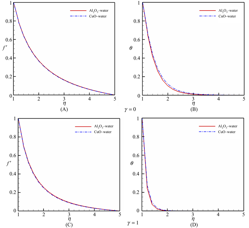
Figure 3.29 (A,C) Velocity profile and (B,D) temperature distribution for different types of nanofluids when ɸ = 0.04, Re = 1, and Pr = 6.8.

Table 3.6

Effects of different kind of nanoparticles on skin friction coefficient when ɸ = 0.04

γ	Re	Nanoparticles
γ	Re	CuO	Al₂O₃
0	0.1	0.679741	0.703897
0	1	1.194617	1.224377
0	2	1.579317	1.615502
1	0.1	0.730548	0.754673
1	1	1.765922	1.793399
1	2	2.82033	2.850088

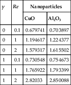
Table 3.7

Effects of different kind of nanoparticles on Nusselt number when ɸ = 0.04

γ	Re	Nanoparticles
γ	Re	CuO	Al₂O₃
0	0.1	1.846686	1.70097
0	1	4.324278	4.113995
0	2	5.996721	5.711652
1	0.1	2.676284	2.540234
1	1	15.23057	15.03967
1	2	28.85855	28.59338

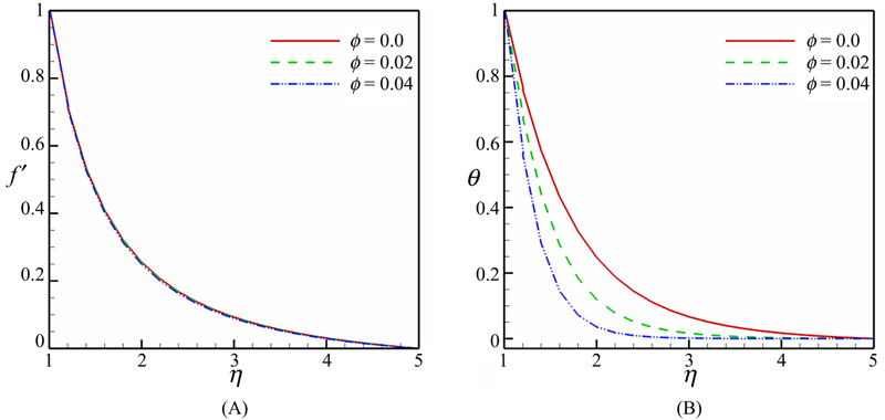
Figure 3.30 Effect of nanoparticle volume fraction (ɸ) on (A) velocity profile and (B) temperature distribution when Re = 1, γ = 1, and Pr = 6.8 (CuO–water).

Figure 3.31 Effect of Reynolds number on (A) velocity profile, (B) pressure distribution, and (C) temperature distribution when ɸ = 0.04, γ = 0, and Pr = 6.8 (CuO–water).

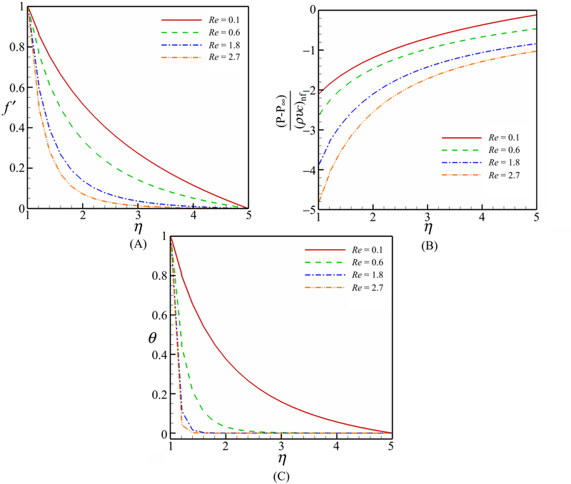
Figure 3.32 Effect of Reynolds number on (A) velocity profile, (B) pressure distribution, and (C) temperature distribution when ɸ = 0.04, γ = 1 and Pr = 6.8 (CuO–water).

Fig. 3.33 shows the effect of suction parameter on the velocity profile, pressure distribution, and temperature distribution. The velocity curves in Fig. 3.33 show that the velocity gradient at the surface increases as γ increases, which implies the increasing of the wall shear stress. The temperature is found to decrease as γ increases, it also decreases as the distance from the surface increases and finally vanishes in a large distance from the surface, which implies an increase in the wall temperature gradient and in turn an increase in the surface heat transfer rate. Hence, the Nusselt number increases as γ increases. Effect of suction parameter on pressure distribution is similar to that of Reynolds number in the presence of suction. Fig. 3.34 shows the effects of the Reynolds number, suction parameter, and nanoparticle volume fraction on the skin friction coefficient. It can be found that the skin friction coefficient decreases with an increase in nanoparticle volume fraction, while it increases with an increase in Reynolds number and suction parameter. Fig. 3.35 depicts the effects of the Reynolds number, suction parameter, and nanoparticle volume fraction on Nusselt number. Nusselt number is an increasing function of Reynolds number, suction parameter, and nanoparticle volume fraction.

Figure 3.33 Effect of suction parameter on (A) velocity profile, (B) pressure distribution, and (C) temperature distribution when ɸ = 0.04, Re = 1, and Pr = 6.8 (CuO–water).

Figure 3.34 (A–B) Effects of the Reynolds number, suction parameter, and nanoparticle volume fraction on skin friction coefficient when Pr = 6.8 (CuO–water).

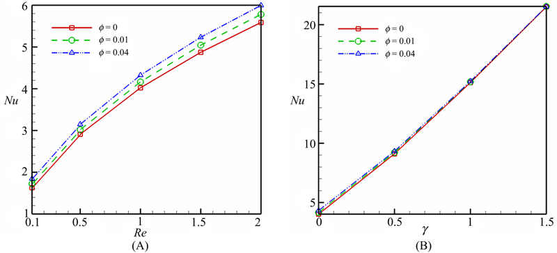
Figure 3.35 (A–B) Effects of the Reynolds number, suction parameter, and nanoparticle volume fraction on Nusselt number when Pr = 6.8 (CuO–water).

..................Content has been hidden....................

You can't read the all page of ebook, please click here login for view all page.

Table of Contents for Chapter 3: Nanofluid Forced Convection Heat Transfer

Create new playlist

Sign In

Sign Up

Abstract

Keywords

3.1. Effect of nonuniform magnetic field on forced convection heat transfer of Fe3O4-water nanofluid

3.1.1. Problem definition

3.1.2. Effects of active parameters

3.2. MHD nanofluid flow and heat transfer considering viscous dissipation

3.2.1. Problem definition and mathematical model

3.2.1.1. Problem definition

3.2.1.2. Numerical method

3.2.2. Effects of active parameters

3.3. Forced convection heat transfer in a semiannulus under the influence of a variable magnetic field

3.3.1. Problem definition

3.3.2. Effects of active parameters

3.4. MHD nanofluid flow and heat transfer considering viscous dissipation

3.4.1. Problem definition and mathematical model

3.4.1.1. Problem definition

3.4.1.2. Numerical method

3.4.2. Effects of active parameters

Table of Contents for
Chapter 3: Nanofluid Forced Convection Heat Transfer

3.1. Effect of nonuniform magnetic field on forced convection heat transfer of Fe₃O₄-water nanofluid