
7.3. Magnetic nanofluid forced convective heat transfer in the existence of variable magnetic field using two-phase model
7.3.1. Problem definition
The schematic diagram and the mesh of the semiannulus enclosure used in the present CVFEM program are shown in Fig. 7.16 [7]. The inner wall is maintained at constant temperatures Th and the other walls are maintained at constant temperature Tc (Th > Tc). The boundary conditions for concentration are similar to those of temperature. For the expression of the magnetic field strength, it can be considered that the magnetic source represents a magnetic wire placed vertically to the x–y plane at the point  . The components of the magnetic field intensity
  and the magnetic field strength
  can be considered as [3]:

Figure 7.16 Geometry and the boundary conditions.
 (7.40)
 (7.41)
 (7.42)
where γ′ is the magnetic field strength at the source (of the wire) and  is the position where the source is located. The contours of the magnetic field strength are shown in Fig. 7.17. In this chapter, magnetic source is located at (−0.01 cols, 0.5 rows). The upper wall is Lid-driven with velocity of ULid. In this section, γ is equal to 45°.

Figure 7.17 Contours of the (A) magnetic field strength H; (B) magnetic field intensity component in x-direction Hx; (C) magnetic field intensity component in y-direction Hy.
The continuity, momentum under Boussinesq approximation, and energy equations for the laminar and steady-state natural convection in a two-dimensional enclosure can be written in dimensional form as follows:
 (7.43)
 (7.44)
 (7.45)
 (7.46)
 (7.47)
The stream function and vorticity are defined as follows:
 (7.48)
The following nondimensional variables should be introduced:
 (7.49)
By using these dimensionless parameters, the equations become:
 (7.50)
 (7.51)
 (7.52)
 (7.53)
where Prandtl number, the Brownian motion parameter, the thermophoretic parameter, Lewis number, Hartmann number, Eckert number, and Reynolds number are defined as: Pr = μ/ρfα, 

 , and
, and  , respectively.
, respectively.The local Nusselt number of the nanofluid along the hot wall can be expressed as:
 (7.54)
where r is the radial direction. The average Nusselt number on the hot circular wall is evaluated as:
 (7.55)
The heatlines are adequate tools for visualization and analysis of two-dimensional convection heat transfer, through an extension of the heat flux line concept to include the advection terms. Heat function (H) is defined in terms of the energy equation as follows:
 (7.56)
7.3.2. Effects of active parameters
In this section, forced convection heat transfer of ferrofluid in the presence of variable magnetic field is investigated using CVFEM. Two-phase model is used to simulate nanofluid. Calculations are made for various values of Reynolds numbers (Re = 10, 100, and 500), Lewis number (Le = 2, 4, and 8), and Hartmann number (Ha = 0, 5, 10, and 20). In all calculations, the Pr, ɛ1, and Ec are set to 6.8, 0.0, and 10−5, respectively.
The effects of Reynolds number and Hartmann number on isotherms, streamlines, isoconcentration, and heatline contours are shown in Figs. 7.18–7.20. At low Reynolds number, one main eddy exists in streamline. By increasing Reynolds number, another small eddy generates near the bottom wall. As Reynolds number increases up to 500, the second eddy become stronger. So, the enclosure divides into two regions with respect to ζ = 22.5°.
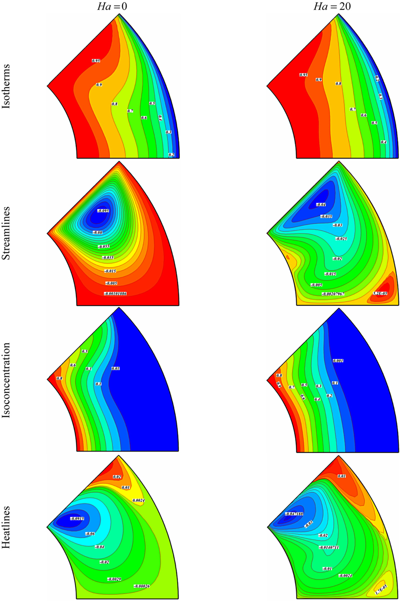
Figure 7.18 Comparison of the isotherms, streamlines, isoconcentration, and heatline contours for different values of Hartmann number when Le = 4, Nt = Nb = 0.5, Re = 10, and Pr = 6.85.

Figure 7.19 Comparison of the isotherms, streamlines, isoconcentration, and heatline contours for different values of Hartmann number when Le = 4, Nt = Nb = 0.5, Re = 100, and Pr = 6.85.

Figure 7.20 Comparison of the isotherms, streamlines, isoconcentration, and heatline contours for different values of Hartmann number when Le = 4, Nt = Nb = 0.5, Re = 500, and Pr = 6.85.
Due to the existence of two eddies which rotate in reverse direction, thermal plume appears to generate near the hot wall. As Hartmann number increases, Lorentz forces suppress the flow and diminish the thermal plume. Isoconcentration becomes more distributed in high Reynolds number, and this effect is reduced in the presence of magnetic field. Heatline contours have two regions in low Reynolds number, while it has three regions in high Reynolds number. Applying magnetic field leads to generate a small passive region at the bottom right corner.
Figs. 7.21 and 7.22 show the effects of Hartmann number, Reynolds number, and Lewis number on local and average Nusselt number. As Reynolds number increases, thermal boundary layer thickness near the hot wall decreases and in turn the rate of heat transfer increases with the increase of Reynolds number. As Hartmann number increases, Lorentz forces become stronger and suppress the flow. So, thermal boundary layer thickness increases with the increase of Hartmann number and in turn the Nusselt number decreases with the increase of Hartmann number. Increasing Lewis number leads to the decrease in rate of heat transfer. Due to the existence of thermal plume, maximum or minimum point appears in the local Nusselt number profile.

Figure 7.21 Effects of Hartmann number, Reynolds number, and Lewis number on local Nusselt number Nuloc along hot wall.

Figure 7.22 Effects of Hartmann number, Reynolds number, and Lewis number on average Nusselt number Nuave along hot wall.
7.4. Nonuniform magnetic field effect on nanofluid hydrothermal treatment considering Brownian motion and thermophoresis effects
7.4.1. Problem definition
The physical model along with the important geometrical parameters and the mesh of the enclosure used in the present CVFEM program are shown in Fig. 7.23 [8]. The inner wall is maintained at constant heat flux. The outer wall is maintained at constant temperature Th. The inner and outer walls are maintained at constant concentration Ch and Cc, respectively. The shape of inner cylinder profile is assumed to mimic the following pattern:

Figure 7.23 (A) Geometry and the boundary conditions; (B) the mesh of enclosure considered in this work.
in which rin is the base circle radius, rout is the radius of outer cylinder, A and N are amplitude and number of undulations, respectively, and ζ is the rotation angle. In this chapter, A and N equal to 0.2 and 4, respectively. The contours of the magnetic field strength are shown in Fig. 7.24. In this chapter, magnetic source is located at (−0.05 cols, 0.5 rows).

Figure 7.24 Contours of the (A) magnetic field strength H; (B) magnetic field intensity component in x-direction Hx; (C) magnetic field intensity component in y-direction Hy.
The nanofluid’s density ρ is as follows:
 (7.58)
where ρf is the base fluid’s density, Tc is a reference temperature,  is the base fluid’s density at the reference temperature, and β is the volumetric coefficient of expansion. Taking the density of base fluid as that of the nanofluid, the density becomes
where ρ0 is the nanofluid’s density at the reference temperature.
The continuity, momentum under Boussinesq approximation, and energy equations for the laminar and steady-state natural convection in a two-dimensional enclosure can be written in dimensional form as follows [8]:
(7.60)
 (7.61)
 (7.62)
 (7.63)
(7.64)For the variation of the magnetization M, with the magnetic field intensity  and temperature T, the following relation derived experimentally in [3] is considered:
where K′ is a constant and  is the Curie temperature.
In the aforementioned equations, μ0 is the magnetic permeability of vacuum (4π × 10−7 Tm/A), is the magnetic field strength,  is the magnetic induction
  , and the bar above the quantities denotes that they are dimensional.
The stream function and vorticity are defined as follows:
(7.66)Also, the following nondimensional variables should be introduced:
 (7.67)
By using these dimensionless parameters, the equations become:
 (7.68)
 (7.69)
 (7.70)
(7.71)where thermal Rayleigh number, the buoyancy ratio number, Prandtl number, the Brownian motion parameter, the thermophoretic parameter, Lewis number, Hartmann number, Eckert number, and Magnetic number arising from FHD of nanofluid are defined as:  ,
,  ,
,  ,
,  ,
,  ,
,  , and
, and  , respectively.
The local Nusselt number of the nanofluid along the inner wall can be expressed as:
 (7.72)
The average Nusselt number on the hot wall is evaluated as:
 (7.73)
7.4.2. Effects of active parameters
Natural convection heat transfer in an enclosure filled with nanofluid external magnetic field is investigated numerically. The effects of Rayleigh number (Ra = 103, 104, and 105), buoyancy ratio number (Nr = 0.1 and 4), Hartmann number (Ha = 0, 2, 6, and 10), and Lewis number (Le = 2 and 4) on flow and heat transfer characteristics are examined. In all calculations, the Pr, ɛ1, Ec, Brownian motion parameter (Nb), and thermophoretic parameter of nanofluid (Nt) are set to 6.85, 0.0, 10−6, 0.5, and 0.5, respectively.
The effects of Hartmann number, Rayleigh number, buoyancy ratio number, and Lewis number on isotherms, streamlines, isoconcentration, and heatline contours are shown in Figs. 7.25–7.28. At Ra = 103 the conduction heat transfer mechanism is more pronounced. For this reason, the isotherms are parallel to each other. As Ra increases, the distribution of isotherm contours increases. At Ra = 103, two equal eddies exist which are symmetric withrespect to ζ = 45°. The strength of upper eddy increases with the increase of Hartmann number.

Figure 7.25 Comparison of the isotherms, streamlines, isoconcentration, and heatline contours for different values of Hartmann number when Nr = 0.1, Le = 2, Nt = Nb = 0.5, Ra = 103, MnF = 5, and Pr = 6.85.
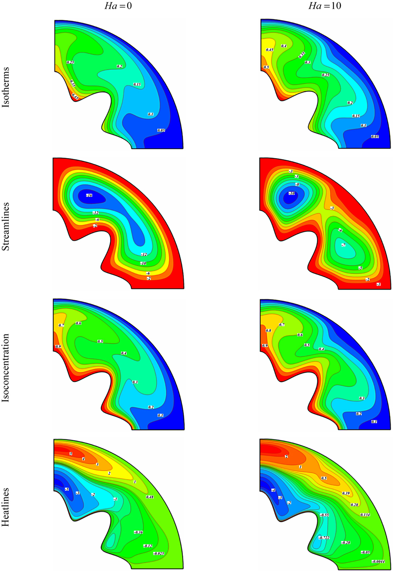
Figure 7.26 Comparison of the isotherms, streamlines, isoconcentration, and heatline contours for different values of Hartmann number when Nr = 0.1, Le = 2, Nt = Nb = 0.5, Ra = 105, MnF = 5, and Pr = 6.85.

Figure 7.27 Comparison of the isotherms, streamlines, isoconcentration, and heatline contours for different values of Hartmann number when Nr = 4, Le = 2, Nt = Nb = 0.5, Ra = 105, MnF = 5, and Pr = 6.85.

Figure 7.28 Comparison of the isotherms, streamlines, isoconcentration, and heatline contours for different values of Hartmann number when Nr = 0.1, Le = 4, Nt = Nb = 0.5, Ra = 105, MnF = 5, and Pr = 6.85.
With the increase of Ra, the role of convection in heat transfer becomes more significant. Also, it can be seen that as Ra increases the distribution of isoconcentration contours increases. The heat flow within the enclosure is displayed using the heat function obtained from conductive heat fluxes (∂Θ/∂X, ∂Θ/∂Y) as well as convective heat fluxes (VΘ, UΘ). Heatlines emanate from hot regimes and end on cold regimes illustrating the path of heat flow. The domination of conduction heat transfer in low Rayleigh number can be observed from the heatline patterns because no passive area exists. The increase of Ra causes the clustering of heatlines from hot to the cold wall and generates passive heat transfer area in which heat is rotated without having significant effect on heat transfer between walls. By increasing buoyancy ratio, a small eddy which is rotated clockwise appears near the vertical wall. This eddy disappears by increasing Hartmann number. As Hartmann number increases, the Lorentz forces increase and in turn the nanofluid flow suppressed. So, thermal boundary layer thickness increases with the increase of Lorentz forces. As Rayleigh number increases, the buoyancy forces increases and in turn thermal boundary layer thickness near the hot wall decreases. Similar trend is observed for buoyancy ratio number and Lewis number.
The effects of Hartmann number, Rayleigh number, buoyancy ratio number, and Lewis number on local Nusselt number are shown in Fig. 7.29. The profiles of the Nuloc profiles have local extremes, which are related to the thermal plumes and crest over the inner cylinder. Also, it can be found that the local Nusselt number decreases with the increase of Hartmann number. Fig. 7.30 shows the effect of Hartmann number, Rayleigh number, buoyancy ratio number, and Lewis number on average Nusselt number. The average Nusselt number increases with the increase of Rayleigh number, buoyancy ratio number, and Lewis number, while it decreases with the increase of Hartmann number.
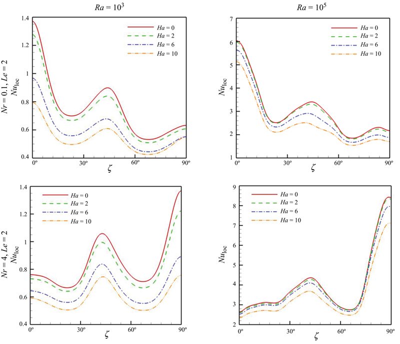
Figure 7.29 Effects of Hartmann number, Rayleigh number, buoyancy ratio number, and Lewis number on local Nusselt number Nuloc along cold wall.

Figure 7.30 Effects of Hartmann number, Rayleigh number, buoyancy ratio number, and Lewis number on average Nusselt number.
7.5. Ferrofluid-mixed convection heat transfer in the existence of variable magnetic field
7.5.1. Problem definition
The schematic diagram and the mesh of the semiannulus enclosure used in the present CVFEM program are shown in Fig. 7.31 [9]. The inner wall is maintained at constant temperatures Th and the other walls are maintained at constant temperature Tc (Th > Tc). For the expression of the magnetic field strength, it can be considered that the magnetic source represents a magnetic wire placed vertically to the x–y plane at the point  . The contours of the magnetic field strength are shown in Fig. 7.32. In this chapter, magnetic source is located at (−0.01 cols, 0.5 rows). The upper wall is Lid-driven with velocity of ULid.

Figure 7.31 (A) Geometry and the boundary conditions; (B) the mesh of enclosure considered in this work.

Figure 7.32 Contours of the (A) magnetic field strength H; (B) magnetic field intensity component in x-direction Hx; (C) magnetic field intensity component in y-direction Hy.
The flow is two-dimensional, laminar, and incompressible. The magnetic Reynolds number is assumed to be small, so that the induced magnetic field can be neglected compared with the applied magnetic field. The flow is considered to be steady, two-dimensional, and laminar. Using the Boussinesq approximation, the governing equations of heat transfer and fluid flow for nanofluid can be obtained as follows:
(7.74)
 (7.75)
 (7.76)
 (7.77)
where  , the variation of magnetic field-dependent (MFD) viscosity (δ) has been taken to be isotropic, δ1 = δ2 = δ3= δ. For the variation of the magnetization M, with the magnetic field intensity and temperature T, the following relation, derived experimentally in [3] and also used in [4], is considered:
where K′ is a constant and is the Curie temperature.
In the aforementioned equations, μ0 is the magnetic permeability of vacuum (4π × 10−7 Tm/A), is the magnetic field strength, is the magnetic induction , and the bar above the quantities denotes that they are dimensional.
The effective density, heat capacitance, thermal diffusivity, thermal expansion coefficient, dynamic viscosity, and effective electrical conductivity of the nanofluid are defined as:
 (7.84)
 (7.85)
By introducing the following nondimensional variables:
 (7.86)
Using the dimensionless parameters, the equations now become:
 (7.87)
 (7.88)
 (7.89)
 (7.90)
where  ,
,  ,
,  , and
, and  are the Reynolds number, Grashof number, Hartmann number arising from MHD, temperature number, Eckert number, Richardson number, viscosity parameter, and Magnetic number arising from FHD the for the base fluid, respectively. The stream function and vorticity are defined as:
, , and
 (7.91)
The stream function satisfies the continuity Eq. (7.87). The vorticity equation is obtained by eliminating the pressure between the two momentum equations, that is, by taking y-derivative of Eq. (7.88) and subtracting from it the x-derivative of Eq. (7.89). The boundary conditions as shown in Fig. 7.31 are as follows:
 (7.92)
The values of vorticity on the boundary of the enclosure can be obtained using the stream function formulation and the known velocity conditions during the iterative solution procedure. The local Nusselt number of the nanofluid along the hot wall can be expressed as:
 (7.93)
(7.94)7.5.2. Effects of active parameters
In this section, mixed convection heat transfer of ferrofluid in the presence of variable magnetic field is investigated using CVFEM. Also, the effect of MFD viscosity on hydrothermal behavior is considered. Calculations are made for various values of volume fraction of nanoparticles (ɸ = 0 and 4%), Richardson numbers (Ri =0.001, 1, and 10), Magnetic number (MnF = 0, 2, 4, 6, and 10), Hartmann number (Ha = 0, 5, and 10), and viscosity parameter (δ* = 0, 0.2, 0.4, and 0.6). In all calculations, the Pr, ɛ1, Ec and Reynolds number (Re) are set to 6.8, 0.0, 10−5, and 100, respectively.
Comparison of the streamlines between nanofluid and pure fluid is shown in Fig. 7.33. The velocity components of nanofluid are increased because of an increase in the energy transport in the fluid with the increase of volume fraction. Thermal boundary layer thickness decreases with the increase of nanofluid volume fraction. Isotherm and streamline contours for different values of viscosity parameter, Richardson, Hartmann, and Magnetic numbers are shown in Figs. 7.34–7.36. When Ri = 0.01, the heat transfer in the enclosure is mainly dominated by the conduction mode. At MnF = 0 and Ha = 0, the streamlines show one rotating eddy.

Figure 7.33 Comparison of the streamlines between nanofluid (ɸ = 0.04) (– – –) and pure fluid (ɸ = 0) (––) when Ri = 10, Re = 100, MnF = 10, Ha = 10, Ec = 10−5, ɛ1 = 0, δ* = 0, Pr = 6.8.

Figure 7.34 Isotherms (left) and streamlines (right) contours for different values of Richardson number and Magnetic number when Ha = 0, δ* = 0.

Figure 7.35 Isotherms (up) and streamlines (down) contours for different values of Richardson number when MnF = 0, Ha = 10, δ* = 0.

Figure 7.36 Isotherms (left) and streamlines (right) contours for different values of δ*, Ha, and MnF when Ri = 10.
When Hartmann number increases a small vortex generates near the magnetic source, so thermal plume appears in this region. As magnetic number increases, the main vortex turns into two smaller vortexes and in turn reverse thermal plume appears near the location of magnetic source. As Richardson number increases, the role of convection in heat transfer becomes more significant. At Ri = 10, the center of main vortex moves downward and thermal boundary layer thickness near the inner wall becomes thinner. When Hartmann and Magnetic numbers increase up to 10, the main vortex turns into three eddies. Three thermal plumes generate over the inner wall due to the existence of eddies which rotate in different directions. Also, it can be seen that as viscosity parameter increases, thermal boundary layer thickness decreases and one counter clockwise eddy generates at center of the enclosure.
Fig. 7.37 depicts that the effects of Magnetic number, Hartmann number, viscosity parameter, and Richardson number on average Nusselt number. Thermal boundary layer thickness increases with the increase of Magnetic number and Hartmann number, while it decreases with the augment of Richardson number. So, the average Nusselt number increases with the increase of Richardson number, while it decreases with the increase of Hartmann number and Magnetic number. Also, it can be concluded that by considering the effect of magnetic field on viscosity of the fluid, the rate of heat transfer increases.

Figure 7.37 Effects of Ha, MnF, Ri, and δ* on average Nusselt number Nuave along hot wall.
7.6. Influence of magnetic field on heat transfer of magnetic nanofluid in a sinusoidal double pipe heat exchanger
7.6.1. Problem definition
Fig. 7.38A illustrates the three-dimensional schematic of the sinusoidal double pipe heat exchanger in the presence of the wire parallel to axis of heat exchanger [10]. The magnetic field is generated by an electric current going through a thin and straight wire oriented parallel to the longitudinal axis (z) at the position (a, b) and the current in the wire flows in the direction of positive z-axis. The structure of the magnetic field in vicinity of the wire is depicted in the Fig. 7.38B. Fig. 7.39 illustrates the geometry of a sinusoidal two-tube heat exchanger with length L and the height of inner tubedi, that is, amplitude (δ) and wavelength (Lw). The total length of wavy wall is six wavelengths, that is, there are six waves along wavy-wall. For the current study, the following dimensionless geometric parameters are applied; wavy amplitude (A) is assumed 0, 0.1, 0.2, and 0.3 in this study. In addition, the profile of the lower wavy-wall can be represented by:

Figure 7.38 (A) Three-dimensional sinusoidal double-tube heat exchanger with magnetic field carrying wire; (B) the effect of magnetic field intensity on the ferrofluid of inside the inner pipe of heat exchanger.

Figure 7.39 Two-dimensional sinusoidal double-tube heat exchanger without magnetic field carrying wire.
 (7.95)
In this section, Navier–Stokes equations and energy equations are coupled to obtain heat transfer inside the sinusoidal double-tube heat exchanger. To investigate the influence of the magnetic field, the components of the magnetic field should be accounted in the momentum equations. Moreover, it is assumed that physical properties of the fluid are constant. The effects of magnetic fields on the viscosity and the thermal conductivity of the ferrofluid have been assumed to be negligible. It should be mentioned that the nonuniform transverse magnetic field has a negligible effect in MHD, and the Lorentz force is also considered negligible compared with the magnetic force due to the electrical conductivity.
Considering these assumptions, the dimensional conservation equations for steady state condition are as follows.
Continuity equation:
 (7.96)
Momentum equation:
 (7.97)
 (7.98)
 (7.99)
Energy equation:
 (7.100)
The terms FK(x) and FK(y) are related to FHD due to the existence of the magnetic gradient and are called the Kelvin force.  and
and  are the components of Kelvin force in the x- and y-directions, respectively. They are resulted from the electric current flowing through the wire. Therefore, it is needed to define the magnetic field of electric current. The components of the magnetic field Hx, Hy in the x-and y-directions are calculated as follows [3]:
and are the components of Kelvin force in the x- and y-directions, respectively. They are resulted from the electric current flowing through the wire. Therefore, it is needed to define the magnetic field of electric current. The components of the magnetic field Hx, Hy in the x-and y-directions are calculated as follows [3]:
 (7.101)
 (7.102)
The magnetic field strength is given by
 (7.103)
It is needed to be mentioned that the term  should be added to the momentum equation in the z-direction when axial nonuniform magnetic gradient is existed in the domain. M is the magnetization and is defined as [11]
should be added to the momentum equation in the z-direction when axial nonuniform magnetic gradient is existed in the domain. M is the magnetization and is defined as [11]
 (7.104)
The unit cell of the crystal structure of magnetite has a volume of about 730 A3 and contains eight molecules of Fe3O4, each of them having a magnetic moment of 4μB [12]. Therefore, the particle magnetic moment for the magnetite particles is obtained as
 (7.105)
Also, ξ is the Langevin parameter and is defined as [11]
 (7.106)
It is also noted that dimensionless magnet number (Mn) is used to measure and the effect of the magnetic field intensity. Magnetic number (Mn) is dependent to the magnetic field intensity. This means that Mn increases with an increase in the magnetic field intensity.
 (7.107)
where χ is the magnetic susceptibility of ferrofluid. As mentioned earlier, the magnetic susceptibility of a ferrofluid containing 4 vol.% with a mean diameter of 10 nm is in the order of χ = 0.348586 [12]. Hr is the characteristic of magnetic field strength and calculated by  . The mixture and physical properties in the aforementioned equations are calculated as follows.
. The mixture and physical properties in the aforementioned equations are calculated as follows.The Reynolds number and the Nusselt number, as two main nondimensional numbers, are calculated by the following equation:
 (7.108)
 (7.109)
where Tb is bulk temperature and  is expressed by following equation:
In the present study, the second-order upwind numerical scheme decoupling with the SIMPLEC algorithm is used, and all the governing equations are solved through a finite volume CFD in-house code.
The inflow conditions of ferrofluid are equivalent to Rem = 100 and 50, and the Reynolds number of air flow is Reair = 2300. Also, for studying heat transfer, results of Nusselt number have been presented for water-based ferrofluid containing of 4 vol.% Fe3O4 spherical shape particles with 10 nm mean diameter. Boundary conditions were applied to the ferrofluid inflow (inlet velocity) with constant temperature (Thot,in = T0) and air flow as cold gas (inlet velocity) with constant temperature (Tcold,in = T0). FVM has been used in this problem. In recent decade, several authors presented new powerful numerical methods [13–29].
7.6.2. Effects of active parameters
The effects of different parameters like Reynolds number, magnetic number, and geometric shape coefficient on the heat transfer of ferrofluid are comprehensively studied. The effects of different geometric configurations (four types) of inner pipe with ferrofluid flow are investigated in the nonuniform magnetic field. Fig. 7.40 illustrates streamlines for two cavities in different geometric shapes. Production of eddies as a result of separation in cavities results in an increase in the heat transfer rate. As an adverse pressure gradient is formed as a result of geometric nonuniformity (i.e., sinusoidal shape), the separation is clearly discerned in the domain.

Figure 7.40 Streamlines for two cavities of sinusoidal pipe in Rem = 50: (A) A = 0.1, (B) A = 0.2, and (C) A = 0.3.
Fig. 7.41 represents the Nusselt number along the inner tube for various geometrical shapes under different magnetic number. It can be seen that nonuniform magnetic field enhances velocity gradient near the wall and hence results in an increase in the Nusselt number. This observation is due to restarting flow because of the existence of Lorentz forces.
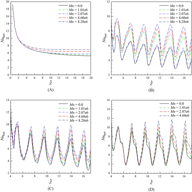
Figure 7.41 Effect Nusselt number for Rem = 50 and values of geometric factor: (A) A = 0, (B) A = 0.1, (C) A = 0.2, and (D) A = 0.3.
Fig. 7.42 represents the Nusselt number for geometric coefficient and different Reynolds numbers. The figure shows that the effects of Reynolds number are more in maximum Nusselt number. Moreover, an increase in Reynolds number results in an increase in the Nusselt number. The Nusselt number has a periodically decreasing behavior from the beginning of the sinusoidal part of the pipe. Also, increasing Reynolds number moves the separation point toward the crest of the sinus wave in diverging part of the pipe. Electrical wire produces a nonuniform magnetic field in x- and y-directions. This field is perpendicular to ferrofliud flow direction. As a magnetic field intensity is increased, the force to flow in cross planes increases. This increase results in a secondary flow, which appears as two eddies. Fig. 7.43 illustrates streamlines in the presence of nonuniform magnetic field at plane on A = 0, z* = 15.5. These eddies diffuse ferrofluid toward the wall in x–y plane. Two eddies are symmetric with respect to the y-axis. It can be seen that streamlines recede from electrical wire as a result of Kelvin force. Fig. 7.44 illustrates the temperature distribution on plane at z* = 15.5 for simple double pipe heat exchanger (A = 0) with Rem = 50. It can be observed that magnetic field causes cold boundary layer to extend toward the center of inner pipe and the magnetic field intensification increases this extension.

Figure 7.42 Effect of Nusselt number for different Reynolds in geometric factor: (A) A = 0, (B) A = 0.1, (C) A = 0.2, and (D) A = 0.3.

Figure 7.43 Streamlines for Rem = 50 and geometric factor A = 0 in z* = 15.5.

Figure 7.44 Nondimensional temperature profile in Rem = 50, z* = 15.5, and geometric factor A = 0: (A) Mn = 0, (B) Mn = 1.01 × 10⁶, (C) Mn = 2.07 × 10⁶, (D) Mn = 4.60 × 10⁶, (E) Mn = 8.28 × 10⁶, and (F) Mn = 18.64 × 10⁶.
Fig. 7.45 shows the temperature distribution for sinusoidal pipe (A = 0.1) at the plane z* = 15.5. The comparison of Figs. 7.44 and 7.45 indicates that the effect of magnetic field in A = 0.1 is less than A = 0. According to Eq. (7.107), the intensity of a magnetic field has an inverse relation with the distance from electrical wire. In A = 0.1 due to a sinusoidal wall of the pipe, the distance between the wire and the centerline of the pipe increases and the magnetic field intensity decreases. Fig. 7.46 compares the effect of geometric shape factor on heat flux (the Nusselt number) for Rem = 50. In converging section of the inner tube, the Nusselt number increases due to the increase in temperature gradient. On the contrary, the Nusselt number decreases in the diverging section due to a reduction in temperature gradient. Fig. 7.47 illustrates the variation of friction coefficient along the inner tube at Rem = 100. The friction coefficient increases due to the increase of magnetic field intensity along the tube. In higher shape coefficient, this increase is not as intense as the Nusselt number increases due to the magnetic field intensity. Fig. 7.48 presents axial velocity distribution at A = 0, z* = 15.5, and for different magnetic field intensities in Rem = 50. It can be seen that increase in magnetic field causes ferrofluid to go toward the inner tube wall.

Figure 7.45 Nondimensional temperature profile in Rem = 50, z* = 15.5, and geometric factor A = 0.1: (A) Mn = 0, (B) Mn = 1.01 × 10⁶, (C) Mn = 2.07 × 10⁶, (D) Mn = 4.60 × 10⁶, (E) Mn = 8.28 × 10⁶, (F) Mn = 18.64 × 10⁶.

Figure 7.46 Effect Nusselt number in different values geometric factor in case Mn = 2.07 × 10⁶ and Rem = 50.

Figure 7.47 Effect friction factor in Reynolds number Rem = 100 and different values of geometric factor: (A) A = 0, (B) A = 0.1, (C) A = 0.2, and (D) A = 0.3.

Figure 7.48 The effect of nonuniform crossover magnetic field on nondimensional axial velocity distribution of ferrofluid (three dimension) for Rem = 50, z* = 15.5, and geometric factor A = 0: (A) Mn = 0, (B) Mn = 1.01 × 10⁶, (C) Mn = 2.07 × 10⁶, (D) Mn = 4.60 × 10⁶, (E) Mn = 8.28 × 10⁶, and (F) Mn = 18.64 × 10⁶.
The effect of geometric shape on average Nusselt number is presented in Fig. 7.49 for Mn = 0 and Rem = 100. As expected, with increase in shape coefficient, averaged Nusselt number increases due to the sinusoidal shape of inner tube. Fig. 7.50 illustrates the variation temperature distribution along the x-direction for different shape coefficients at Rem = 100. It is found that magnetic field increases the velocity gradient in the vicinity of the tube wall and this increase results in the extension of the cold boundary layer toward ferrofluid. So, ferrofluids temperature decreases at the centerline of inner tube and heat transfer improves. Fig. 7.51 depicts nondimensional temperature contour in various sections along the sinusoidal double pipe (A = 0.2) in the presence of magnetic field (Mn = 2.07 × 10⁶). In the axial direction, cold boundary layer extends toward centerline of the pipe and intensifies heat transfer. Fig. 7.52 indicates nondimensional temperature along the heat exchanger for different shape coefficient at Rem = 100. The results show that the magnetic field decreases the outlet temperature of ferrofluid. Fig. 7.53 compares the effect of magnetic field on the ratio of the Nusselt number in different shape coefficients. This ratio is defined as the ratio of mean Nusselt number in the presence of a magnetic field to the Nusselt number without magnetic field. It is noticed that this ratio significantly increases as magnetic field intensity increases in ferrofluid in constant Reynolds number.

Figure 7.49 The effect of geometric form factor on average Nusselt in Rem = 100.

Figure 7.50 The effect of geometric of magnetic field in dimensionless temperature for Rem = 50, z* = 15.5, y* = 1, and geometric factor: (A) A = 0, (B) A = 0.1, (C) A = 0.2, and (D) A = 0.

Figure 7.51 Nondimensional temperature contour in six sinusiodal wave sections inside the inner tube, for A = 0.2 and Mn = 2.07 × 10⁶: (A) z* = 4.55, (B) z* = 6.75, (C) z* = 8.95, (D) z* = 11.15, (E) z* = 13.35, and (F) z* = 15.5.

Figure 7.52 The effect of magnetic field in nondimensional temperature in along the axis of heat exchanger for Rem = 50 with different values of geometric factor: (A) A = 0, (B) A = 0.1, (C) A = 0.2, and (D) A = 0.3.

Figure 7.53 The ratio of average Nusselt number of ferrofluid for Rem = 50 in various intensities of magnetic field with different geometric factors.
..................Content has been hidden....................
You can't read the all page of ebook, please click here login for view all page.