
Chapter 7
Nanofluid Flow and Heat Transfer in the Presence of Variable Magnetic Field
Abstract
Magnetic nanofluid (ferrofluid) is a magnetic colloidal suspension consisting of base liquid and magnetic nanoparticles with a size range of 5–15 nm in diameter coated with a surfactant layer. The effect of magnetic field on fluids is worth investigating due to its numerous applications in a wide range of fields. The study of interaction of the magnetic field or the electromagnetic field with fluids have been documented, for example, among nuclear fusion, chemical engineering, medicine, and transformer cooling. The goal of nanofluid is to achieve the highest possible thermal properties at the smallest possible concentrations by uniform dispersion and stable suspension of nanoparticles in host fluids. In this chapter, the influence of external magnetic field on ferrofluid flow and heat transfer is investigated. The effects of both ferrohydrodynamic and magnetohydrodynamic have been taken in to account. So, the effects of Lorentz and Kelvin forces on hydrothermal behavior are examined.
Keywords
ferrofluid
ferrohydrodynamic
Kelvin force
Lorentz force
Joule heating
7.1. Effect of space dependent magnetic field on free convection of Fe3O4–water nanofluid
7.1.1. Problem definition
The physical model along with the important geometrical parameters and the mesh of the enclosure used in the present control volume-based finite element method (CVFEM) program are shown in Fig. 7.1 [1]. The inner circular wall is maintained at constant hot temperature Th, the two horizontal walls are thermally isolated, and other walls are maintained at constant cold temperature Tc (Th > Tc). To reach the shape of inner circular and outer rectangular boundary which consists of the right and top walls, a supper elliptic function can be used as follows:

Figure 7.1 (A) Geometry and the boundary conditions; (B) the mesh of enclosure considered in this work.
 (7.1)
(7.1)When a = b and n = 1, the geometry becomes a circle. As n increases from 1, the geometry would approach a rectangle for a ≠ b and square for a = b. In this chapter, we assumed that rin/rout = 0.6.
For the expression of the magnetic field strength, it can be considered that two magnetic sources at points  and
and  . The components of the magnetic field intensity
  and the magnetic field strength
  can be considered as [2]:
 (7.2)
(7.2)
 (7.3)
(7.3)
 (7.4)
(7.4)where γ is the magnetic field strength at the source (of the wire). The contours of the magnetic field strength are shown in Fig. 7.2. In this chapter, magnetic source is located at  and
and  .
.

Figure 7.2 Contours of the (A) magnetic field strength H; (B) magnetic field intensity component in x-direction Hx; (C) magnetic field intensity component in y-direction Hy.
The flow is two-dimensional, laminar, and incompressible. The magnetic Reynolds number is assumed to be small, so that the induced magnetic field can be neglected compared with the applied magnetic field. Using the Boussinesq approximation, the governing equations of heat transfer and fluid flow for nanofluid can be obtained as follows:
 (7.5)
(7.5)
 (7.6)
(7.6)
 (7.7)
(7.7)
 (7.8)
(7.8)The terms  and
and  in (7.6) and (7.7), respectively, represent the components of magnetic force, per unit volume, and depend on the existence of the magnetic gradient on the corresponding x- and y-directions. These two terms are well known from ferrohydrodynamic (FHD) which is the so-called Kelvin force. The terms
  and
and  appearing in (7.6) and (7.7), respectively, represent the Lorentz force per unit volume toward the x- and y-directions and arise due to the electrical conductivity of the fluid. These two terms are known in magnetohydrodynamic (MHD). The principles of MHD and FHD are combined in the mathematical model presented in [3] and the aforementioned terms arise together in the governing Eqs. (7.6) and (7.7). The term
  in Eq. (7.8) represents the thermal power per unit volume due to the magnetocaloric effect. Also, the term
  in (7.8) represents the Joule heating. For the variation of the magnetization M, with the magnetic field intensity
  and temperature T, the following relation is used [4]:
and in (7.6) and (7.7), respectively, represent the components of magnetic force, per unit volume, and depend on the existence of the magnetic gradient on the corresponding x- and y-directions. These two terms are well known from ferrohydrodynamic (FHD) which is the so-called Kelvin force. The terms in Eq. (7.8) represents the thermal power per unit volume due to the magnetocaloric effect. Also, the term
where K′ is a constant and  is the Curie temperature.
In the aforementioned equations, μ0 is the magnetic permeability of vacuum (4π × 10−7 Tm/A), is the magnetic field strength,  is the magnetic induction
  , and the bar above the quantities denotes that they are dimensional. The effective density (ρnf) and heat capacitance (ρCp)nf of the nanofluid are defined as:
where ɸ is the solid volume fraction of nanoparticles. Thermal diffusivity of the nanofluid is as follows:
 (7.12)
and the thermal expansion coefficient of the nanofluid can be determined as
The dynamic viscosity of the nanofluids is given as
 (7.14)
The effective thermal conductivity of the nanofluid can be approximated by the Maxwell–Garnetts model as [1]:
 (7.15)
and the effective electrical conductivity of nanofluid was presented as follows:
 (7.16)
By introducing the following nondimensional variables:
 (7.17)
 and L = rout − rin. Using the dimensionless parameters, the equations now become:
 (7.18)
 (7.19)
 (7.20)
 (7.21)
where  ,
,  , and
, and  are the Rayleigh number, Prandtl number, Hartmann number arising from MHD, temperature number, curie temperature number, Eckert number, and Magnetic number arising from FHD the for the base fluid, respectively. The thermophysical properties of the nanofluid are given in Table 7.1 [3].
Table 7.1
Thermophysical properties of water and nanoparticles [3]
| ρ (kg/m3) | Cp (J/kg k) | k (W/m k) | β × 105 (K) | σ (Ω/m) | |
| Pure water | 997.1 | 4179 | 0.613 | 21 | 0.05 |
| Fe3O4 | 5200 | 670 | 6 | 1.3 | 25000 |

The stream function and vorticity are defined as:
 (7.22)
The stream function satisfies the continuity Eq. (7.18). The vorticity equation is obtained by eliminating the pressure between the two momentum equations, that is, by taking y-derivative of Eq. (7.20) and subtracting from it the x-derivative of Eq. (7.19).
The boundary conditions as shown in Fig. 7.1 are as follows:
 (7.23)
The values of vorticity on the boundary of the enclosure can be obtained using the stream function formulation and the known velocity conditions during the iterative solution procedure.
The local Nusselt number of the nanofluid along the hot wall can be expressed as:
 (7.24)
where r is the radial direction. The average Nusselt number on the hot circular wall is evaluated as:
 (7.25)
To estimate the enhancement of heat transfer between the case of ɸ = 0.04 and the pure fluid (base fluid) case, the heat transfer enhancement is defined as:
 (7.26)
7.1.2. Effects of active parameters
In this work, the effects of FHD and MHDs on Fe3O4–water flow and heat transfer are investigated numerically using the CVFEM. Calculations are made for various values of volume fraction of nanoparticles (ɸ = 0.0 and 0.04), Rayleigh numbers (Ra = 103, 104, and 105), Magnetic number arising from FHD (MnF = 0, 20, 60, and 100), and Hartmann number arising from MHD (Ha = 0.5 and 10). In all calculations, the Prandtl number (Pr), temperature number (ɛ1), and Eckert number (Ec) are set to 6.8, 0.0, and 1.0e−6, respectively.
Fig. 7.3 shows the comparison of the isotherms and streamlines between nanofluid and pure fluid. The velocity components of nanofluid are enhanced because of an augment in the energy transport in the fluid with the increase of volume fraction. Thus, the absolute values of stream functions increase with increasing the volume fraction of nanofluid. Also, it can be seen that thermal boundary layer thickness around the hot wall increases with the increase of nanoparticle volume fraction.

Figure 7.3 Comparison of the isotherms and streamlines between nanofluid (ɸ = 0.04) (– – –) and pure fluid (ɸ = 0) (––) when Pr = 6.8.
Fig. 7.4 depicts the effects of Rayleigh number, Hartmann number, and Magnetic number on isotherms and streamlines. |Ψmax| increases with the increase of Rayleigh number, while it decreases with the augment of Hartmann number and Magnetic number. When Ra = 103, the heat transfer in the enclosure is mainly dominated by the conduction mode. At the absence of magnetic field, the streamlines show one rotating eddy. When Magnetic parameter increases, another vortex appears near the center line which rotates in the reverse direction in comparison with the primary vortex. Lorentz force has no significant effect on isotherm and streamline in low Rayleigh number. As the Rayleigh number increases up to 104, the role of convection in heat transfer becomes more important and consequently the thermal boundary layer on the surface of the inner wall becomes thinner. In addition, a plume starts to appear on the top of the inner circular wall. It is interesting to remark that at MnF = 100 and Ha = 10, the smaller primary vortex turns into two smaller eddies near the magnetic sources. At Ra = 105, two reverse plumes are observed in the absence of FHD and MHD effects. As Hartmann number increases, one of the plumes disappears due to Lorentz forces.

Figure 7.4 Isotherms (left) and streamlines (right) contours for different values of Rayleigh number, Hartmann number, and Magnetic number when Pr = 6.8, ɸ = 0.04.
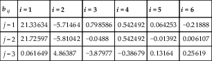
Fig. 7.5 shows the effects of Magnetic number, Hartmann number, and Rayleigh number on local Nusselt number along the hot wall. As Hartmann number increases, the Nusselt number decreases, but the opposite trend is observed for Magnetic number and Rayleigh number. The existence of maximum and minimum points in the local Nusselt number profile corresponds to the presence of thermal plumes. Fig. 7.6A–C shows the effects of Hartmann number and Rayleigh number on average Nusselt number along hot wall. The effects of Magnetic number, Rayleigh number, and Hartmann number on heat transfer enhancement are shown in Fig. 7.6D–F. The corresponding polynomial representations for Nusselt number and enhancement in heat transfer are as follows:

Figure 7.5 Effects of Magnetic number, Hartmann number, and Rayleigh number on local Nusselt number Nuloc along hot wall when Pr = 6.8, ɸ = 0.04.
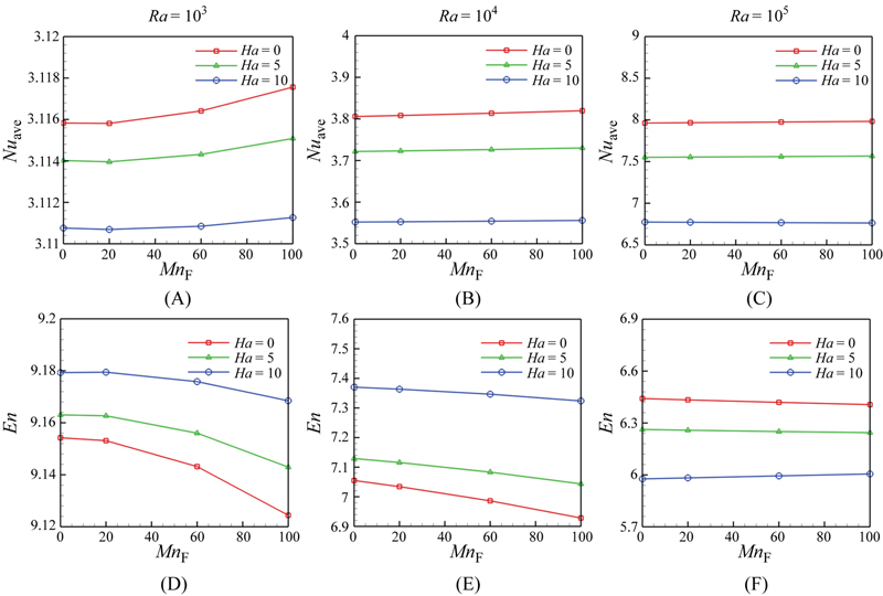
Figure 7.6 (A–C) Effects of Magnetic parameter, Hartmann number, and Rayleigh number on average Nusselt number Nuave along hot wall when Pr = 6.8, ɸ = 0.04; (D–F) effects of Magnetic number, Rayleigh number, and Hartmann number on heat transfer enhancement when Pr = 6.8.
 (7.27)
 (7.28)
Table 7.2
Constant coefficient for using Eq. (7.27)
| aij | i = 1 | i = 2 | i = 3 | i = 4 | i = 5 | i = 6 |
| j = 1 | 19.51647 | −10.0868 | −0.00804 | 1.525112 | 0.001086 | 0.003349 |
| j = 2 | 19.53085 | −0.87952 | −10.1291 | −0.03518 | 1.525112 | 2.186806 |
| j = 3 | −0.29704 | 1.107821 | 0.654435 | −0.00017 | 0.041509 | −0.24967 |
| j = 4 | −0.15202 | 0.647229 | 1.043281 | 0.044365 | 0.005999 | −0.24883 |
| j = 5 | −0.07156 | 0.161803 | 0.861233 | 1.818237 | 1.846604 | −3.66821 |
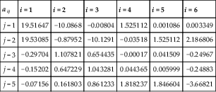
Table 7.3
Constant coefficient for using Eq. (7.28)
| bij | i = 1 | i = 2 | i = 3 | i = 4 | i = 5 | i = 6 |
| j = 1 | 21.33634 | −5.71464 | 0.798586 | 0.542492 | 0.064253 | −0.21888 |
| j = 2 | 21.72597 | −5.81042 | −0.0488 | 0.542492 | −0.01392 | 0.006107 |
| j = 3 | 0.061649 | 4.86387 | −3.87977 | −0.38679 | 0.13164 | 0.25619 |
As Buoyancy force (due to temperature gradient) and Kelvin force (due to external nonuniform magnetic field) increase, the rate of heat transfer increases, but the opposite trend is observed for Lorentz forces. It means that increasing Lorentz forces lead to the decrease of Nusselt number. Also, it can be concluded that the effect of Magnetic parameter on Nuave is more pounced at low Rayleigh number. At low Rayleigh number, heat transfer enhancement increases with the increase of Hartmann number, but the opposite trend is observed for Magnetic parameter. At high Rayleigh number, Magnetic parameter has no significant effect on enhancement, but increasing Hartmann number causes the heat transfer enhancement to decrease. The effect of nanoparticles is more pronounced at low Rayleigh number than at high Rayleigh number due to the domination of conduction heat transfer mechanism.
7.2. Simulation of ferrofluid flow for magnetic drug targeting using lattice Boltzmann method
7.2.1. Problem definition
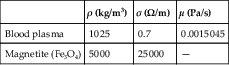
The steady, two-dimensional, incompressible, laminar flow is considered taking place in a channel. The width of channel is D and the length of the channel is L, such that L/D = 25. The flow at the entrance is assumed to be fully developed  (Fig. 7.7A) [5]. The flow is subjected to a magnetic source, which is placed very close to the lower plate and below it (a = 0.25L, b = −0.1D) (Fig. 7.8). The fluid in vessel is considered a homogenous mixture of Fe3O4–blood plasma. Thermophysical properties of the nanoscale ferromagnetic particle and blood plasma are assumed to be constant (Table 7.4).
(Fig. 7.7A) [5]. The flow is subjected to a magnetic source, which is placed very close to the lower plate and below it (a = 0.25L, b = −0.1D) (Fig. 7.8). The fluid in vessel is considered a homogenous mixture of Fe3O4–blood plasma. Thermophysical properties of the nanoscale ferromagnetic particle and blood plasma are assumed to be constant (Table 7.4).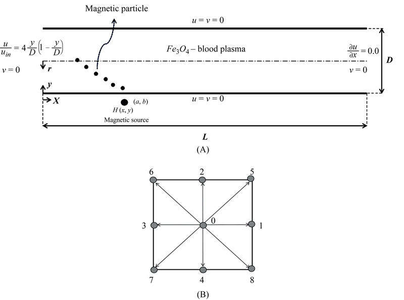
Figure 7.7 (A) Geometry of the vessel; (B) discrete velocity set of two-dimensional nine velocity.

Figure 7.8 Contours of the magnetic field strength H.
Table 7.4
Thermophysical properties of blood plasma and magnetite
| ρ (kg/m3) | σ (Ω/m) | μ (Pa/s) | |
| Blood plasma | 1025 | 0.7 | 0.0015045 |
| Magnetite (Fe3O4) | 5000 | 25000 | — |
The components of the magnetic field intensity (Hx, Hy) and the magnetic field strength (H) can be considered as [3]:
 (7.29)
 (7.30)
 (7.31)
One of the novel computational fluid dynamics (CFD) methods, which solves the Boltzmann equation to simulate the flow instead of solving the Navier–Stokes equations, is called lattice Boltzmann methods (LBM). LBM has several advantages such as simple calculation procedure and efficient implementation for parallel computation, over other conventional CFD methods, because of its particulate nature and local dynamics. The LB model uses one distribution function f for the flow. It uses modeling of movement of fluid particles to capture macroscopic fluid quantities such as velocity and pressure. In this approach, the fluid domain is discretized to uniform Cartesian cells. Each cell holds a fixed number of distribution functions, which represent the number of fluid particles moving in these discrete directions. The D2Q9 model [6] was used and values of  for |c0| = 0 (for the static particle),
  for |c1–4| = 1, and
  for
for  are assigned in this model (Fig. 7.7B). The density and distribution functions are calculated by solving the lattice Boltzmann equation, which is a special discretization of the kinetic Boltzmann equation. After introducing BGK approximation, the general form of lattice Boltzmann equation with external force is as follows.
For the flow field:
 (7.32)
where ∆t denotes lattice time step, ci is the discrete lattice velocity in direction i, Fk is the external force in direction of lattice velocity, and  denotes the lattice relaxation time for the flow. The kinetic viscosity υ is defined in terms of its respective relaxation times, that is,
  . Note that the limitation 0.5 < τ should be satisfied for both relaxation times to ensure that viscosity and thermal diffusivity are positive. Furthermore, the local equilibrium distribution function determines the type of problem that needs to be solved. It also models the equilibrium distribution functions, which are calculated with Eq. (7.32) for flow field, respectively.
 (7.33)
where  is a weighting factor and ρ is the lattice fluid density.
To incorporate buoyancy forces and magnetic forces in the model, the force term in the Eq. (7.32) needs to calculate as follows:
 (7.34)
where A and B are  and
and  , respectively.
  , and
, and  are Reynolds number, Hartmann number, and Magnetic number arising from FHD [3].
and , and are Reynolds number, Hartmann number, and Magnetic number arising from FHD [3].Finally, macroscopic variables calculate with the following formula:
 (7.35)
To simulate the nanofluid by the LBM, because of the interparticle potentials and other forces on the nanoparticles, the nanofluid behaves differently from the pure liquid from the mesoscopic point of view and is of higher efficiency in energy transport as well as better stabilization than the common solid–liquid mixture. For modeling the nanofluid because of changing in the fluid density, viscosity, and electrical conductivity, some of the governed equations should change. The effective density (ρnf), the effective viscosity (μnf), and electrical conductivity (σ)nf of the nanofluid are defined as:
 (7.37)
(7.38)with ɸ being the volume fraction of the nanoscale ferromagnetic particle (Fe3O4) and subscripts nf, s, and f stand for the mixture, nanoscale ferromagnetic particle (Fe3O4), and the carrier fluid (blood plasma), respectively.
The local and average skin friction coefficient is defined as follows:
 (7.39)
7.2.2. Effects of active parameters
Targeted drug delivery system under the influence of an applied magnetic field is studied. The working fluid is a homogenous mixture of magnetite in blood plasma. Lattice Boltzmann method scheme was utilized to obtain the numerical simulation. The effects of Reynolds number (Re = 50, 100, 200, and 400) and Magnetic number (MnF = 0, 20, 60, and 100) on streamline, velocity profile, and skin friction coefficient are examined for constant values of volume fraction of nanoparticle (ɸ = 0.04) and Hartmann number (Ha = 20).
The effects of Magnetic number and Reynolds number on streamlines are shown in Figs. 7.9–7.12. In the absence of the magnetic field (MnF = 0), the streamlines are straight lines. As Reynolds number increases, velocity boundary layer thickness decreases. In the presence of the magnetic field, a clockwise vortex appears at the area where the magnetic source is placed. This vortex causes perturbation in the flow pattern and nanofluid flow recirculation may occur in this region. This phenomenon is more pronounced for higher values of Magnetic number.

Figure 7.9 Effect of Magnetic number on streamlines when Re = 50, Ha = 20, ɸ = 0.04.

Figure 7.10 Effect of Magnetic number on streamlines when Re = 100, Ha = 20, ɸ = 0.04.
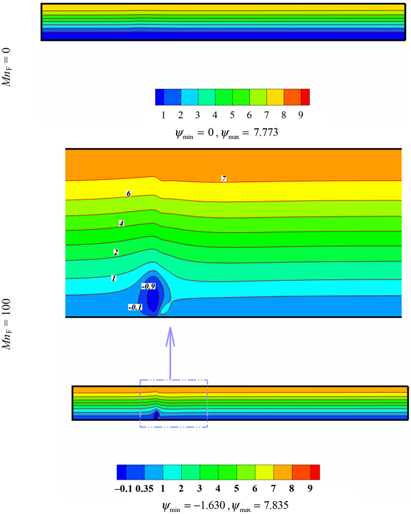
Figure 7.11 Effect of Magnetic number on streamlines when Re = 200, Ha = 20, ɸ = 0.04.

Figure 7.12 Effect of Magnetic number on streamlines when Re = 400, Ha = 20, ɸ = 0.04.
Fig. 7.13 shows the effects of Magnetic number and Reynolds number on velocity profile at x = 0.25L. At x = 0.25L flow is separated from the bottom wall and then reattaches with the lower plate. Finally, the flow at the outlet is again reverted to be fully developed. This phenomenon is more pronounced for higher values of Reynolds number. The effects of Magnetic number and Reynolds number on local skin friction coefficient along the lower and upper walls are shown in Fig. 7.14. The value of local skin friction coefficient at the lower wall increases rapidly near x = 0.2L, where it reaches its maximum value. Very close to the region where the source is located x = 0.25L, a corresponding decrement takes place and at x = 0.25L this parameter takes its minimum negative value.  increases near the area of the magnetic source in a smoother way, and its sign does not change as happens with the lower plate where reverse of the flow occurs. The wall shear is more influenced on the lower plate, below of which the magnetic source is located. It is an interesting observation that there are two points with zero values of skin friction for lower plate. In these points there is no skin friction, and this result may be exciting in the case of creation of fibrinoid. Fig. 7.15 shows the effects of Magnetic number and Reynolds number on average skin friction coefficient. The drag acting on the upper plate is greater than that of the lower. Average skin friction coefficient decreases with the increase of Reynolds number and Magnetic number.
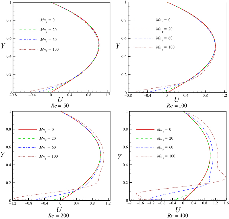
Figure 7.13 Effects of Magnetic number and Reynolds number on velocity profile at x = 0.25L when Ha = 20, ɸ = 0.04.

Figure 7.14 Effects of Magnetic number and Reynolds number on local skin friction coefficient along the (A) lower and (B) upper plates when Ha = 20, ɸ = 0.04.

Figure 7.15 Effects of Magnetic number and Reynolds number on average skin friction coefficient along the (A) lower and (B) upper plates when Ha = 20, ɸ = 0.04.
..................Content has been hidden....................
You can't read the all page of ebook, please click here login for view all page.