
4.4. Ferrofluid flow and heat transfer in a semiannulus enclosure in the presence of magnetic source considering thermal radiation
4.4.1. Problem definition
The schematic diagram and the mesh of the semiannulus enclosure used in the present CVFEM program are shown in Fig. 4.18 [8]. The inner wall is under constant heat flux (q″) and outer wall is maintained at constant temperature (Tc), while the two other walls are thermally insulated. In this study, γ equals to 45°. For the expression of the magnetic field strength, it can be considered that the magnetic source represents a magnetic wire placed vertically to the x–y plane at the point  . The components of the magnetic field intensity
  and the magnetic field strength
  can be considered as [9]:
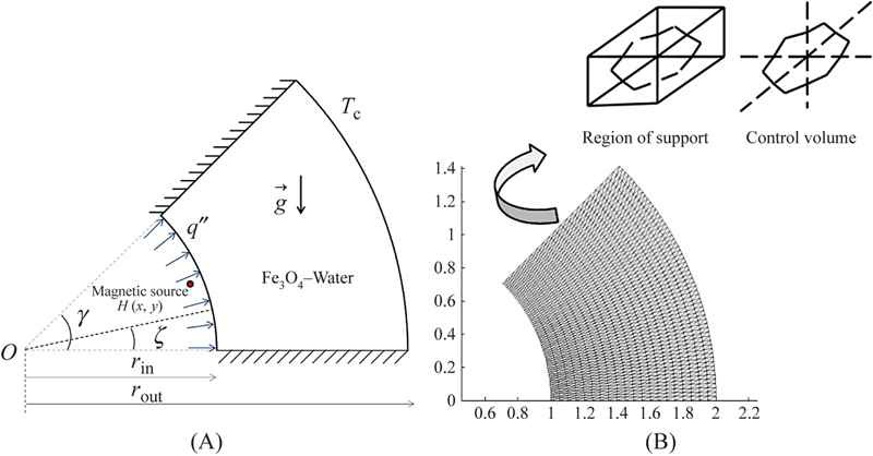
Figure 4.18 (A) Geometry and the boundary conditions; (B) the mesh of enclosure considered in this work.
 (4.56)
 (4.57)
 (4.58)
where γ′ is the magnetic field strength at the source (of the wire) and (a, b) is the position where the source is located. The contours of the magnetic field strength are shown in Fig. 4.19. In this section, magnetic source is located at (−0.05, 0.5).
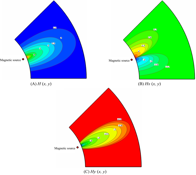
Figure 4.19 Contours of the (A) magnetic field strength H; (B) magnetic field intensity component in x-direction Hx; (C) magnetic field intensity component in y-direction Hy.
The flow is considered to be steady, two-dimensional, incompressible, and laminar. Using the Boussinesq approximation, the governing equations of heat transfer and fluid flow for nanofluid can be obtained as follows [9]:
 (4.59)
 (4.60)
 (4.61)
 (4.62)
where the radiation heat flux qr is considered according to Rosseland approximation such that  where σe and βR are the Stefan–Boltzmann constant and the mean absorption coefficient, respectively. Following Raptis [2], the fluid-phase temperature differences within the flow are assumed to be sufficiently small, so that T4 may be expressed as a linear function of temperature. This is done by expanding T4 in a Taylor series about the temperature Tc and neglecting higher order terms to yield,
  .
.
where σe and βR are the Stefan–Boltzmann constant and the mean absorption coefficient, respectively. Following Raptis [2], the fluid-phase temperature differences within the flow are assumed to be sufficiently small, so that T4 may be expressed as a linear function of temperature. This is done by expanding T4 in a Taylor series about the temperature Tc and neglecting higher order terms to yield, The terms  and
and  in (4.60) and (4.61), respectively, represent the components of magnetic force, per unit volume, and depend on the existence of the magnetic gradient on the corresponding x- and y-directions. These two terms are well known from FHD which is the so-called Kelvin force. The terms
  and
and  appearing in (4.60) and (4.61), respectively, represent the Lorentz force per unit volume toward the x- and y-directions and arise due to the electrical conductivity of the fluid. These two terms are known in MHD. The principles of MHD and FHD are combined in the mathematical model presented in [9] and the earlier-mentioned terms arise together in the governing Eqs. (4.60) and (4.61). The term
  in Eq. (4.62) represents the thermal power per unit volume due to the magneto caloric effect. Also, the term
  in (4.62) represents the Joule heating. For the variation of the magnetization M, with the magnetic field intensity
  and temperature T, the following relation derived in [9] is considered:
and in (4.60) and (4.61), respectively, represent the components of magnetic force, per unit volume, and depend on the existence of the magnetic gradient on the corresponding x- and y-directions. These two terms are well known from FHD which is the so-called Kelvin force. The terms in Eq. (4.62) represents the thermal power per unit volume due to the magneto caloric effect. Also, the term
where K′ is a constant and  is the Curie temperature.
In the above equations, μ0 is the magnetic permeability of vacuum (4π × 10−7Tm/A), is the magnetic field strength,  is the magnetic induction
  , and the bar above the quantities denotes that they are dimensional: (ρnf), (ρCp), (αnf), (βnf), (μnf), (knf), and (σnf) are defined as:
 (4.66)
 (4.68)
 (4.69)
 (4.70)
The stream function satisfies the continuity Eq. (4.59). By introducing the following nondimensional variables:
 (4.71)
Using the dimensionless parameters, the equations now become:
 (4.72)
 (4.73)
 (4.74)
 (4.75)
where  ,
,  ,
,  ,
,  ,
,  , and
, and  are the Rayleigh number, Prandtl number, Hartmann number arising from MHD, temperature number, Eckert number, magnetic number arising from FHD the for the base fluid, and radiation parameter, respectively.
The stream function and vorticity are defined as:
 (4.76)
The stream function satisfies the continuity Eq. (4.72). The vorticity equation is obtained by eliminating the pressure between the two momentum equations, that is, by taking y-derivative of Eq. (4.74) and subtracting from it the x-derivative of Eq. (4.73).
 (4.77)
The values of vorticity on the boundary of the enclosure can be obtained using the stream function formulation and the known velocity conditions during the iterative solution procedure.
The local Nusselt number of the nanofluid along the inner wall can be expressed as:
 (4.78)
where r is the radial direction. The average Nusselt number on the hot circular wall is evaluated as:
 (4.79)
4.4.2. Effects of active parameters
Ferrofluid (Fe3O4–water) flow and heat transfer in a semiannulus enclosure in the presence of an external magnetic field is investigated. CVFEM is used to solve the governing equations. The mathematical model used for the formulation of the problem is consistent with the principles of FHD and MHD. Calculations are made for various values of volume fraction of nanoparticles (ɸ = 0 and 4%), Rayleigh numbers (Ra = 103, 104, and 105), magnetic number arising from FHD (MnF = 0, 20, 60, and 100), radiation parameter (Nr = 0.0 and 0.027), and Hartmann number arising from MHD (Ha = 0, 2, 6, and 10). In all calculations, the Prandtl number (Pr), temperature number (ɛ1), and Eckert number (Ec) are set to 6.8, 0.0, and 1e−5, respectively.
Fig. 4.20 shows the comparison of the isotherm and streamlines between nanofluid and pure fluid. The velocity components of nanofluid are increased because of an increase in the energy transport in the fluid with the increasing of volume fraction. Thus, the absolute values of stream functions indicate that the strength of flow increases with the increase of the volume fraction of nanofluid. Also, it can be found that thermal boundary layer thickness increases with the increase of volume fraction of nanofluid. Fig. 4.21 shows the effect of Hartmann number on isotherm and streamlines. As Hartmann number increases absolute value of maximum stream function decreases. Also, this figure shows that streamlines become more disturb near the magnetic source. Isotherms and streamlines contours for different values of Rayleigh number, Hartmann number, radiation parameter, and magnetic number are shown in Figs. 4.22 and 4.23.
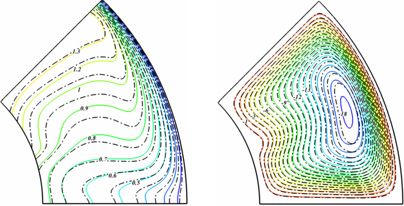
Figure 4.20 Comparison of the isotherm and streamlines between nanofluid (ɸ = 0.04) (––) and pure fluid (ɸ = 0) (– – –) when Nr = 0.027, Ra = 105, MnF = 100, Ha = 10, and Pr = 6.8.
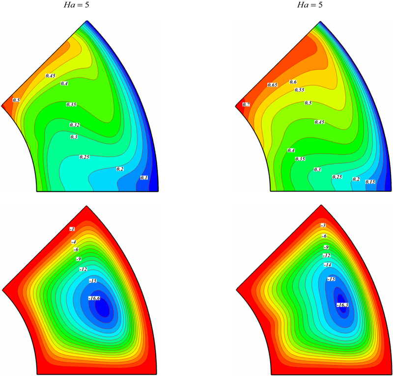
Figure 4.21 Effect of Hartmann number on isotherm and streamlines when Nr = 0.027, Ra = 105, Mn = 100, ɸ = 0.04.

Figure 4.22 Isotherms (up) and streamlines (down) contours for different values of Rayleigh number, Hartmann number, and Magnetic number when Nr = 0.0, ɸ = 0.04, Pr = 6.8.
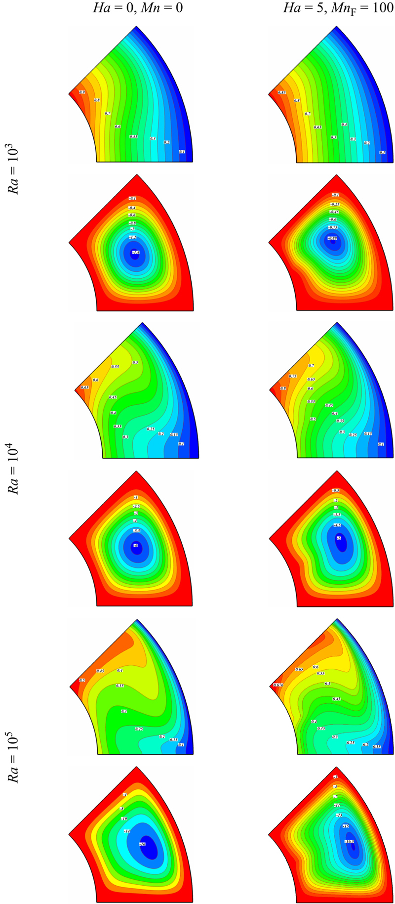
Figure 4.23 Isotherms (up) and streamlines (down) contours for different values of Rayleigh number, Hartmann number, and Magnetic number when Nr = 0.027, ɸ = 0.04, Pr = 6.8.
When Ra = 103, the heat transfer in the enclosure is mainly dominated by the conduction mode. At MnF = 0, Ha = 0 the streamlines show one rotating eddy. In the presence of magnetic field, the vortex center moves upward. As the Rayleigh number increases, the role of convection in heat transfer becomes more significant and consequently the thermal boundary layer thickness on the surface of the inner wall becomes thinner. In addition, a plume starts to appear on the top of the inner circular wall at ζ = 45°. The isotherms and streamlines become denser near the magnetic source (ζ = 22.5°). Also, Fig. 4.23 shows that absolute value of maximum stream function increases with the augment of radiation parameter. The center of the vortex moves downward left by increasing radiation parameter.
Fig. 4.24 depicts that the effects of magnetic number, Hartmann number, radiation parameter, and Rayleigh number on local Nusselt number. Local Nusselt number increases with the increase of Rayleigh number, while it decreases with the increase of Hartmann number and radiation parameter. Local minimum point at ζ = 22.5° in these profiles is related to the existence of magnetic source at this region. The effects of volume fraction of nanofluid, magnetic number, Hartmann number, radiation parameter, and Rayleigh number on average Nusselt number are shown in Fig. 4.25 and Table 4.5. Average Nusselt number increases with the increase of volume fraction of nanofluid, magnetic number, and Rayleigh number, while it decreases with the increase of Hartmann number and radiation parameter.
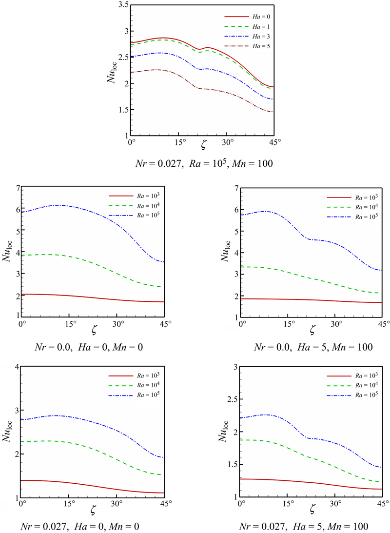
Figure 4.24 Effects of magnetic number, Hartmann number, radiation parameter, and Rayleigh number on local Nusselt number Nuloc along hot wall when ɸ = 0.04.
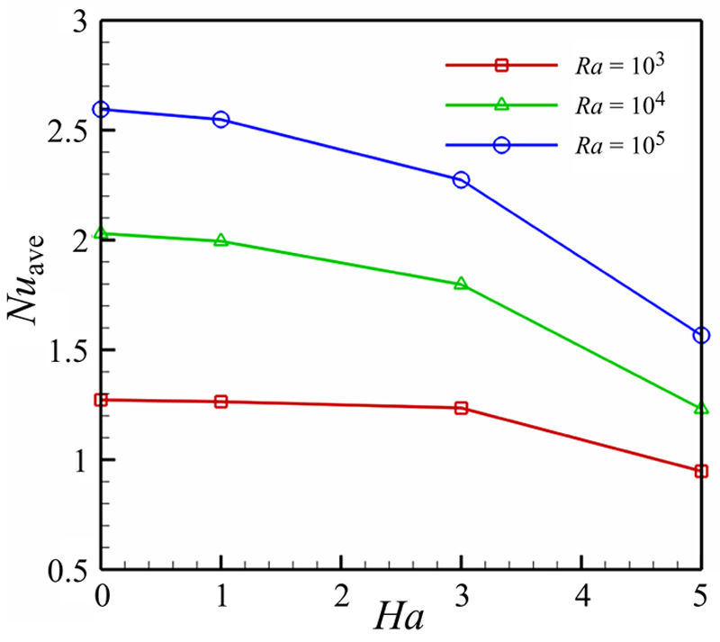
Figure 4.25 Effects of Hartmann number and Rayleigh number on average Nusselt number Nuave along hot wall when Nr = 0.027, ɸ = 0.04.
Table 4.5
Effects of Hartmann number, radiation parameter, nanoparticle volume fraction, and magnetic number on average Nusselt number
| MnF = 0, Ha = 0 | MnF = 100, Ha = 5 | MnF = 100, Ha = 0 | MnF = 0, Ha = 5 | ||||||
| Nr | Nr | Nr | Nr | ||||||
| Ra | ɸ | 0 | 0.027 | 0 | 0.027 | 0 | 0.027 | 0 | 0.027 |
| 103 | 0 | 1.611611 | 0.995565 | 1.519592 | 0.928174 | 1.711999 | 1.010865 | 1.510564 | 0.953924 |
| 103 | 0.04 | 1.890241 | 1.270623 | 1.801949 | 1.215039 | 1.972767 | 1.285426 | 1.796937 | 1.234266 |
| 104 | 0 | 2.906977 | 1.609061 | 2.477273 | 1.244099 | 2.934773 | 1.636442 | 2.459938 | 1.226934 |
| 104 | 0.04 | 3.312842 | 2.022216 | 2.802561 | 1.596926 | 3.34569 | 2.048861 | 2.784897 | 1.582475 |
| 105 | 0 | 4.799285 | 2.103907 | 4.316693 | 1.570677 | 4.775208 | 2.106432 | 4.331907 | 1.564888 |
| 105 | 0.04 | 5.372904 | 2.595023 | 4.789146 | 1.942158 | 5.345175 | 2.588536 | 4.807063 | 1.940414 |

4.5. Nanofluid flow and heat transfer over a stretching porous cylinder considering thermal radiation
4.5.1. Problem definition and mathematical model
4.5.1.1. Problem definition
Consider the steady laminar flow of an incompressible nanofluid caused by a stretching tube with radius a in the axial direction in a fluid at rest as shown in Fig. 4.26, where the z-axis is measured along the axis of the tube and the r-axis is measured in the radial direction [10]. It is assumed that the surface of the tube is at constant temperature Tw and the ambient fluid temperature is T∞ where Tw > T∞. The viscous dissipation is neglected as it is assumed to be small. It is assumed that the base fluid and the nanoparticles are in thermal equilibrium and no slip occurs between them. Under these assumptions, the governing equations are as follows:
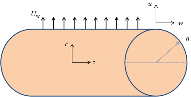
Figure 4.26 Geometry of the problem.
 (4.80)
 (4.81)
 (4.82)
 (4.83)
where the radiation heat flux  is considered according to Rosseland approximation such that where σe and βR are the Stefan–Boltzmann constant and the mean absorption coefficient, respectively. Fluid-phase temperature differences within the flow are assumed to be sufficiently small, so that T4 may be expressed as a linear function of temperature. This is done by expanding T4 in a Taylor series about the temperature T∞ and neglecting higher order terms to yield,
  .
.
where σe and βR are the Stefan–Boltzmann constant and the mean absorption coefficient, respectively. Fluid-phase temperature differences within the flow are assumed to be sufficiently small, so that T4 may be expressed as a linear function of temperature. This is done by expanding T4 in a Taylor series about the temperature T∞ and neglecting higher order terms to yield, The boundary conditions are as follows:
 (4.84)
where  and c is a positive constant. Notice that γ is a constant in which γ > 0 and γ < 0 correspond to mass suction and mass injection, respectively.
The effective density ρnf, the effective dynamic viscosity μnf, the heat capacitance (ρCp)nf, and the thermal conductivity knf of the nanofluid are given as:
 (4.86)
(4.88)Here, ɸ is the nanoparticle volume fraction.
Following [11], we take the similarity transformation:
where prime denotes differentiation with respect to η.
Substituting Eq. (4.89) into Eqs. (4.80) and (4.83), we get the following ordinary differential equations:
 (4.91)
where Re = ca2/2υf is the Reynolds number, υf = μf/ρf is the kinematic viscosity, Pr = μf(ρCp)f/(ρf kf) is the Prandtl number,  is radiation parameter and
  are parameters having the following forms:
 (4.92)
 (4.93)
 (4.94)
The boundary conditions (4.84) become
 (4.95)
The pressure (P) can now be determined from Eq. (4.82) in the form
 (4.96)
 (4.97)
Physical quantities of interest are the skin friction coefficient (Cf) and the Nusselt number (Nu), which are defined as:
 (4.98)
with kf being the thermal conductivity of the base fluid. Furthermore,  and
and  are the surface shear stress and the surface heat flux, respectively, and they are given by
 (4.99)
 (4.100)
that is,
 (4.101)
 (4.102)
Using variables (4.89), we have:
 (4.103)
 (4.104)
4.5.1.2. Numerical method
Before using the Runge–Kutta integration scheme, first we reduce the governing differential equations into a set of first order ODEs [12,13]. Let x1 = η, x2 = f, x3 = f′, x4 = f″, x5 = θ, x6 = θ′. We obtain the following system:
 (4.105)
and the corresponding initial conditions are
 (4.106)
The above nonlinear coupled ODEs along with initial conditions are solved using fourth-order Runge–Kutta integration technique. Suitable values of the unknown initial conditions u1 and u2 are approximated through Newton’s method until the boundary conditions at f′(∞) → 0, θ (∞) → 0 are satisfied. The computations have been performed by using MAPLE. The maximum value of η = ∞, to each group of parameters, is determined when the values of unknown boundary conditions at x = 1 do not change to a successful loop with error less than 10−6. Recently, new numerical methods have been applied for various field of science [14–28].
4.5.2. Effects of active parameters
The effect of thermal radiation on Cu–water nanofluid hydrothermal behavior over a cylinder is studied. The governing equations and their boundary conditions are transformed to ordinary differential equations which are solved numerically using the fourth-order Runge–Kutta integration scheme featuring a shooting technique. Fig. 4.27 shows the effects of nanoparticle volume fraction, Reynolds number, and suction parameter on velocity profile. The momentum boundary layer thickness decreases with the increase of nanoparticle volume fraction. The effects of Reynolds number and suction parameter on momentum boundary layer thickness are similar to that of nanoparticle volume fraction.
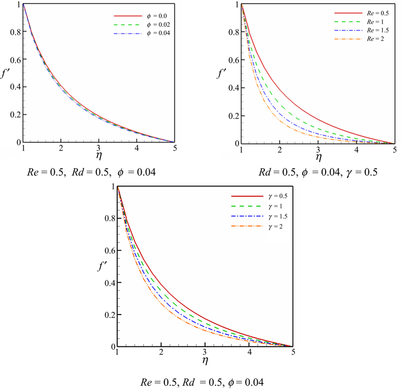
Figure 4.27 Effects of nanoparticle volume fraction, Reynolds number, and suction parameter on velocity profile when Pr = 7.
The effects of nanoparticle volume fraction, Reynolds number, and suction parameter on skin friction coefficient are shown in Fig. 4.28. Skin friction coefficient has direct relationship with Reynolds number and suction parameter, while it has reverse relationship with nanoparticle volume fraction. Fig. 4.29 shows the effects of Reynolds number and suction parameter on pressure distribution. Pressure distribution decreases with the increase of Reynolds number and suction parameter. Fig. 4.30 shows the effects of nanoparticle volume fraction, Reynolds number, suction parameter, and radiation parameter on temperature profile. Thermal boundary layer thickness decreases with the increase of Reynolds number and suction parameter, while it increases with the increase of nanoparticle volume fraction and radiation parameter. Fig. 4.31 shows the effects of nanoparticle volume fraction, Reynolds number, suction parameter, and radiation parameter on Nusselt number. Nusselt number has direct relationship with nanoparticle volume fraction, Reynolds number, suction parameter, and it has reverse relationship with radiation parameter.
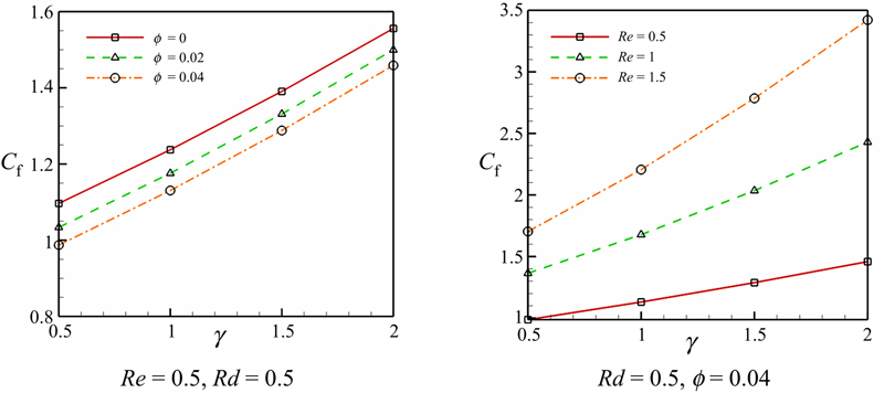
Figure 4.28 Effects of nanoparticle volume fraction, Reynolds number, and suction parameter on skin friction coefficient when Pr = 7.
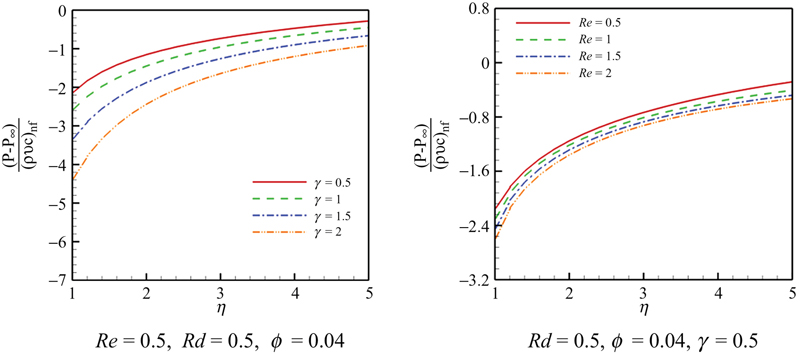
Figure 4.29 Effects of Reynolds number and suction parameter on pressure distribution when Pr = 7.

Figure 4.30 Effects of nanoparticle volume fraction, Reynolds number, suction parameter, and radiation parameter on temperature profile when Pr = 7.

Figure 4.31 Effects of nanoparticle volume fraction, Reynolds number, suction parameter, and radiation parameter on Nusselt number when Pr = 7.
..................Content has been hidden....................
You can't read the all page of ebook, please click here login for view all page.