Search in book...
Toggle Font Controls
Create new playlist

Name your new playlist

Playlist description (optional)
Sign In

Email address

Password

Forgot Password?

or

Continue with Facebook

Continue with Google
Sign Up

Full Name

Email address

Confirm Email Address

Password

or

Continue with Facebook

Continue with Google

Chapter 9

Nanofluid Flow and Heat Transfer in Porous Media

Abstract

The study of convective heat transfer in fluid-saturated porous media has many important applications in technology geothermal energy recovery, such as oil recovery, food processing, fiber and granular insulation, porous burner and heater, combustion of low-calorific fuels to diesel engines, and design of packed bed reactors. Also the flow in porous tubes or channels has been under considerable attention in recent years because of its various applications in biomedical engineering, transpiration cooling boundary layer control, and gaseous diffusion. Nanofluids are produced by dispersing the nanometer-scale solid particles into base liquids with low thermal conductivity, such as water, ethylene glycol, oils. In this chapter, nanofluid hydrothermal behavior in porous media has been investigated.

Keywords

nanofluid

porous media

entropy generation

wall suction/injection

semi analytical method

stagnation point flow

stretching sheet

9.1. Nanofluid heat Transfer over a permeable stretching wall in a porous medium

9.1.1. Problem definition

A steady, constant property, two-dimensional flow of an incompressible nanofluid through a homogenous porous medium with permeability of K, over a stretching surface with linear velocity distribution, that is,

u_{w} = \frac{u_{0} x}{L}

$u_{w} = \frac{u_{0} x}{L}$

is assumed (Fig. 9.1) [1].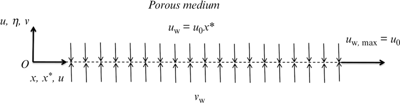

Figure 9.1 Schematic theme of the problem geometry.

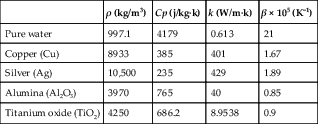
The fluid is a water-based nanofluid containing different types of nanoparticles: Cu, Al₂O₃, Ag, and TiO₂. It is assumed that the base fluid and the nanoparticles are in thermal equilibrium and no slip occurs between them. The thermophysical properties of the nanofluid are given in Table 9.1.

Table 9.1

Thermophysical properties of water and nanoparticles

	ρ (kg/m³)	Cp (j/kg·k)	k (W/m·k)	β × 10⁵ (K⁻¹)
Pure water	997.1	4179	0.613	21
Copper (Cu)	8933	385	401	1.67
Silver (Ag)	10,500	235	429	1.89
Alumina (Al₂O₃)	3970	765	40	0.85
Titanium oxide (TiO₂)	4250	686.2	8.9538	0.9

The transport properties of the medium can be considered independent from the temperature when the temperature difference between wall and ambient is not significant [2]. The origin is kept fixed while the wall is stretching and the y-axis is perpendicular to the surface. Using the aforementioned assumptions, the continuity equation is:

$\frac{\partial u}{\partial x} + \frac{\partial v}{\partial y} = 0$ $\frac{\partial u}{\partial x} + \frac{\partial v}{\partial y} = 0$

(9.1)

Where u and v are velocity components in the x and y directions, respectively. The Brinkman model x-momentum equation reads:

$ρ_{n f} (u \frac{\partial u}{\partial x} + v \frac{\partial v}{\partial y}) = μ_{ef f_{n f}} \frac{\partial^{2} u}{\partial y^{2}} - \frac{μ_{n f}}{K} u$ $ρ_{n f} (u \frac{\partial u}{\partial x} + v \frac{\partial v}{\partial y}) = μ_{ef f_{n f}} \frac{\partial^{2} u}{\partial y^{2}} - \frac{μ_{n f}}{K} u$

(9.2)

$u \frac{\partial T}{\partial x} + v \frac{\partial T}{\partial y} = \frac{k_{n f}}{{(ρ C_{p})}_{n f}} \frac{\partial^{2} T}{\partial y^{2}}$ $u \frac{\partial T}{\partial x} + v \frac{\partial T}{\partial y} = \frac{k_{n f}}{{(ρ C_{p})}_{n f}} \frac{\partial^{2} T}{\partial y^{2}}$

(9.3)

Where

μ_{ef f_{nf}}

$μ_{ef f_{nf}}$

is the effective viscosity which for simplicity in the present study is considered to be identical to the dynamic viscosity, μ_nf. This assumption is reasonable for packed beds of particles [3].

The effective density ρ_nf, the effective dynamic viscosity μ_nf, the heat capacitance (ρC_p)_nf, and the thermal conductivity k_nf of the nanofluid are given as:

$ρ_{n f} = ρ_{f} (1 - φ) + ρ_{s} φ$ $ρ_{n f} = ρ_{f} (1 - φ) + ρ_{s} φ$

(9.4)

$μ_{n f} = \frac{μ_{f}}{{(1 - φ)}^{2.5}}$ $μ_{n f} = \frac{μ_{f}}{{(1 - φ)}^{2.5}}$

(9.5)

${(ρ C_{p})}_{n f} = {(ρ C_{p})}_{f} (1 - φ) + {(ρ C_{p})}_{s} φ$ ${(ρ C_{p})}_{n f} = {(ρ C_{p})}_{f} (1 - φ) + {(ρ C_{p})}_{s} φ$

(9.6)

$\frac{k_{n f}}{k_{f}} = \frac{k_{s} + 2 k_{f} - 2 φ (k_{f} - k_{s})}{k_{s} + 2 k_{f} + 2 φ (k_{f} - k_{s})}$ $\frac{k_{n f}}{k_{f}} = \frac{k_{s} + 2 k_{f} - 2 φ (k_{f} - k_{s})}{k_{s} + 2 k_{f} + 2 φ (k_{f} - k_{s})}$

(9.7)

Here, φ is the solid volume fraction.

The hydrodynamic boundary conditions are:

$u (x^{*}, 0) = u_{0} x^{*}, v (x^{*}, 0) = v_{w}, u (x^{*}, \infty) = 0$ $u (x^{*}, 0) = u_{0} x^{*}, v (x^{*}, 0) = v_{w}, u (x^{*}, \infty) = 0$

(9.8)

Where

x^{*} = x / L

$x^{*} = x / L$

is the nondimensional x-coordinate and L is the length of the porous plate.

The following thermal boundary conditions are considered:

$T (x^{*}, 0) = T_{\infty} + T_{0} {(x^{*})}^{n}, T (x^{*}, \infty) = T_{\infty}$ $T (x^{*}, 0) = T_{\infty} + T_{0} {(x^{*})}^{n}, T (x^{*}, \infty) = T_{\infty}$

(9.9)

$- k_{n f} {\frac{\partial T}{\partial y}|}_{(x^{*}, 0)} = q_{0} {(x^{*})}^{n}, T (x^{*}, \infty) = T_{\infty}$ $- k_{n f} {\frac{\partial T}{\partial y}|}_{(x^{*}, 0)} = q_{0} {(x^{*})}^{n}, T (x^{*}, \infty) = T_{\infty}$

(9.10)

The power-law temperature and heat flux distribution, described in Eqs. (9.9) and (9.10), resent a wider range of thermal boundary conditions including isoflux and isothermal cases. For example, by setting n equal to zero, Eqs. (9.9) and (9.10) yield isothermal and isoflux, respectively.

Second law of thermodynamics analysis of porous media is found to be more complicated compared to the clear fluid counterpart due to increased number of variables in governing equations [4]. In the non-Darcian regime, there are three alternative models for the fluid friction term which are the clear-fluid compatible model, the Darcy model, and the Nield model or the power of drag model. Following the entropy generation function introduced by [4], the volumetric entropy generation rate,

S_{gen}^{•}

$S_{gen}^{•}$

, reads:

$S_{gen} = \frac{k_{n f}}{T^{2}} [{(\frac{\partial T}{\partial x})}^{2} + {(\frac{\partial T}{\partial y})}^{2}] + \frac{μ_{n f}}{T} \{2 [{(\frac{\partial u}{\partial x})}^{2} + {(\frac{\partial u}{\partial y})}^{2}] + {(\frac{\partial u}{\partial x} + \frac{\partial u}{\partial y})}^{2}\} + \frac{μ_{n f}}{T K} (u^{2} + v^{2})$ $S_{gen} = \frac{k_{n f}}{T^{2}} [{(\frac{\partial T}{\partial x})}^{2} + {(\frac{\partial T}{\partial y})}^{2}] + \frac{μ_{n f}}{T} \{2 [{(\frac{\partial u}{\partial x})}^{2} + {(\frac{\partial u}{\partial y})}^{2}] + {(\frac{\partial u}{\partial x} + \frac{\partial u}{\partial y})}^{2}\} + \frac{μ_{n f}}{T K} (u^{2} + v^{2})$

(9.11)

Using boundary layer approximations, Eq. (9.11) reduces to:

$S^{•} = \frac{k_{n f}}{T^{2}} {(\frac{\partial T}{\partial y})}^{2} + \frac{μ_{n f}}{T} {(\frac{\partial u}{\partial y})}^{2} + \frac{μ_{n f}}{T K} u^{2}$ $S^{•} = \frac{k_{n f}}{T^{2}} {(\frac{\partial T}{\partial y})}^{2} + \frac{μ_{n f}}{T} {(\frac{\partial u}{\partial y})}^{2} + \frac{μ_{n f}}{T K} u^{2}$

(9.12)

Using the stream function, ψ(x, y) the continuity equation is satisfied:

$u = \frac{\partial ψ}{\partial y}, v = \frac{\partial ψ}{\partial x}$ $u = \frac{\partial ψ}{\partial y}, v = \frac{\partial ψ}{\partial x}$

(9.13)

The hydrodynamic boundary layer thickness scales with

\sqrt{K}

$\sqrt{K}$

. This can be found through a scale analysis between the first and the second terms on the right hand side of Eq. (9.2), that is, the viscous and the Darcy terms. Therefore, instead of the other similarity parameters reported in the literature, the following dimensionless similarity parameter is defined as:

$η = \frac{y}{\sqrt{K}}$ $η = \frac{y}{\sqrt{K}}$

(9.14)

The u-velocity is assumed to be correlated to f(η), a dimensionless similarity function as:

$u = u_{0} x^{*} f^{'} (η)$ $u = u_{0} x^{*} f^{'} (η)$

(9.15)

Where f’(η) is

\frac{d f}{d η}

$\frac{d f}{d η}$

. Using stream function definition, Eq. (9.15), the stream function and the v-velocity take the following forms:

$v = - \frac{u_{0}}{L} \sqrt{K} f (η), v = u_{0} x^{*} \sqrt{K} f (η)$ $v = - \frac{u_{0}}{L} \sqrt{K} f (η), v = u_{0} x^{*} \sqrt{K} f (η)$

(9.16)

Substituting from u and v into Eqs. (9.2) and (9.4), one will find the following differential equation for the u-momentum equation:

$f^{‴} + Re A_{1} (f f^{″} - {(f')}^{2}) - f^{'} = 0, Re = \frac{ρ_{f} u_{0} K}{L μ_{f}}$ $f^{‴} + Re A_{1} (f f^{″} - {(f')}^{2}) - f^{'} = 0, Re = \frac{ρ_{f} u_{0} K}{L μ_{f}}$

(9.17)

Where A₁ is a parameter having the following form:

$A_{1} = (1 - φ) + \frac{ρ_{s}}{ρ_{f}} φ$ $A_{1} = (1 - φ) + \frac{ρ_{s}}{ρ_{f}} φ$

(9.18)

Where Re is the Reynolds number. Eq. (9.18) should be solved subjected to the following boundary conditions:

$f (0) = \frac{- v_{w} L}{u_{0} \sqrt{K}} = f_{w}, f^{'} (0) = 1, f^{'} (\infty) = 0$ $f (0) = \frac{- v_{w} L}{u_{0} \sqrt{K}} = f_{w}, f^{'} (0) = 1, f^{'} (\infty) = 0$

(9.19)

f_w is the injection parameter. Positive/negative values of f_w show suction/injection into/from the porous surface, respectively.

The wall shear stress is the driving force that drags fluid flow along the stretching wall. The wall shear stress term can then be found, in terms of the similarity function, as:

$τ_{w} = - μ_{n f} {\frac{\partial u}{\partial y}|}_{y = 0} = \frac{- μ_{n f} u_{0} x^{*} f^{″} (0)}{2 \sqrt{K}}$ $τ_{w} = - μ_{n f} {\frac{\partial u}{\partial y}|}_{y = 0} = \frac{- μ_{n f} u_{0} x^{*} f^{″} (0)}{2 \sqrt{K}}$

(9.20)

Introducing a similarity function, θ, as:

$T - T_{\infty} = T_{ref} {(x^{*})}^{n} θ (η)$ $T - T_{\infty} = T_{ref} {(x^{*})}^{n} θ (η)$

(9.21)

Where T_ref is T₀ and

q_{0} \frac{\sqrt{K}}{k}

$q_{0} \frac{\sqrt{K}}{k}$

for the power-law temperature and heat flux boundary conditions, respectively. The thermal energy equation reads:

$θ^{″} + Re ·Pr \cdot \frac{A_{1}}{A_{3}} \cdot A_{2} \cdot {(1 - φ)}^{2.5} (f θ^{'} - n f^{'} θ)) = 0 \Pr = \frac{μ_{f} {(ρ C_{p})}_{f}}{ρ_{f} k_{f}}, Re = \frac{ρ_{f} u_{0} K}{L μ_{f}}$ $θ^{″} + Re ·Pr \cdot \frac{A_{1}}{A_{3}} \cdot A_{2} \cdot {(1 - φ)}^{2.5} (f θ^{'} - n f^{'} θ)) = 0 \Pr = \frac{μ_{f} {(ρ C_{p})}_{f}}{ρ_{f} k_{f}}, Re = \frac{ρ_{f} u_{0} K}{L μ_{f}}$

(9.22)

Where A₂, A₃ are parameters having the following form:

$\begin{array}{l} A_{2} = (1 - φ) + \frac{{(ρ C_{p})}_{s}}{{(ρ C_{p})}_{f}} φ \\ A_{3} = \frac{k_{nf}}{k_{f}} = \frac{k_{s} + 2 k_{f} - 2 φ (k_{f} - k_{s})}{k_{s} + 2 k_{f} + 2 φ (k_{f} - k_{s})} \end{array}$ $\begin{array}{l} A_{2} = (1 - φ) + \frac{{(ρ C_{p})}_{s}}{{(ρ C_{p})}_{f}} φ \\ A_{3} = \frac{k_{nf}}{k_{f}} = \frac{k_{s} + 2 k_{f} - 2 φ (k_{f} - k_{s})}{k_{s} + 2 k_{f} + 2 φ (k_{f} - k_{s})} \end{array}$

(9.23)

Which are subjected to the following boundary conditions:

$\begin{array}{l} θ (0) = 1, θ (\infty) = 0 Power - law temperature \\ θ^{'} (0) = - 1, θ (\infty) = 0 Power - law heat flux \end{array}$ $\begin{array}{l} θ (0) = 1, θ (\infty) = 0 Power - law temperature \\ θ^{'} (0) = - 1, θ (\infty) = 0 Power - law heat flux \end{array}$

(9.24)

For power-law temperature and heat flux boundary conditions, respectively. Employing the definition of convective heat transfer coefficient, the local Nusselt numbers, become:

$N u_{x} = \frac{h x}{k} = \{\begin{cases} \frac{- θ^{'} (0) x}{\sqrt{K}} Power - law temperature \\ \frac{q_{w} x}{K (T_{w} - T_{\infty})} = \frac{x}{θ (0) \sqrt{K}} Power - law heat flux \end{cases}$ $N u_{x} = \frac{h x}{k} = \{\begin{cases} \frac{- θ^{'} (0) x}{\sqrt{K}} Power - law temperature \\ \frac{q_{w} x}{K (T_{w} - T_{\infty})} = \frac{x}{θ (0) \sqrt{K}} Power - law heat flux \end{cases}$

(9.25)

Finally, the local volumetric entropy generation rate for the previous cases, respectively, reads:

$S_{gen}^{•} = HTI+FFI$ $S_{gen}^{•} = HTI+FFI$

(9.26)

Where HTI is the heat transfer irreversibility due to heat transfer in the direction of finite temperature gradients. HTI is common in all types of thermal engineering applications.

The last term (FFI) is the contribution of fluid friction irreversibility to the total entropy generation. Not only the wall and fluid layer shear stress but also the momentum exchange at the solid boundaries (pore level) contributes to FFI. In terms of the primitive variables, HTI and FFI become

$HTI = \{\begin{cases} \frac{A_{3} \cdot k_{f}}{{(θ T_{0} {(x^{*})}^{n} + T_{\infty})}^{2}} {(\frac{θ^{'} T_{0} {(x^{*})}^{n}}{\sqrt{K}})}^{2} Power-law temperature \\ \frac{A_{3} \cdot k_{f}}{{(\frac{θ \sqrt{K} q_{0} {(x^{*})}^{n}}{k + T_{\infty}})}^{2}} {(\frac{θ^{'} q_{0} {(x^{*})}^{n}}{A_{3} \cdot k_{f}})}^{2} Power-law heat flux \end{cases}$ $HTI = \{\begin{cases} \frac{A_{3} \cdot k_{f}}{{(θ T_{0} {(x^{*})}^{n} + T_{\infty})}^{2}} {(\frac{θ^{'} T_{0} {(x^{*})}^{n}}{\sqrt{K}})}^{2} Power-law temperature \\ \frac{A_{3} \cdot k_{f}}{{(\frac{θ \sqrt{K} q_{0} {(x^{*})}^{n}}{k + T_{\infty}})}^{2}} {(\frac{θ^{'} q_{0} {(x^{*})}^{n}}{A_{3} \cdot k_{f}})}^{2} Power-law heat flux \end{cases}$

(9.27)

$FFI = \{\begin{cases} \frac{μ_{f} \cdot {(1 - φ)}^{2.5}}{(θ T_{0} {(x^{*})}^{n} + T_{\infty})} [{(\frac{f^{″} u_{0} x^{*}}{\sqrt{K}})}^{2} + {(\frac{f^{'} u_{0} x^{*}}{\sqrt{K}})}^{2}] Power-law temperature \\ \frac{μ_{f} \cdot {(1 - φ)}^{2.5}}{(\frac{θ \sqrt{K} q_{0} {(x^{*})}^{n}}{k + T_{\infty}})} [{(\frac{f^{″} u_{0} x^{*}}{\sqrt{K}})}^{2} + {(\frac{f^{'} u_{0} x^{*}}{\sqrt{K}})}^{2}] Power-law heat flux \end{cases}$ $FFI = \{\begin{cases} \frac{μ_{f} \cdot {(1 - φ)}^{2.5}}{(θ T_{0} {(x^{*})}^{n} + T_{\infty})} [{(\frac{f^{″} u_{0} x^{*}}{\sqrt{K}})}^{2} + {(\frac{f^{'} u_{0} x^{*}}{\sqrt{K}})}^{2}] Power-law temperature \\ \frac{μ_{f} \cdot {(1 - φ)}^{2.5}}{(\frac{θ \sqrt{K} q_{0} {(x^{*})}^{n}}{k + T_{\infty}})} [{(\frac{f^{″} u_{0} x^{*}}{\sqrt{K}})}^{2} + {(\frac{f^{'} u_{0} x^{*}}{\sqrt{K}})}^{2}] Power-law heat flux \end{cases}$

(9.28)

Where T_∞ and T₀ are measured in degrees of Kelvin.

One can also define the Bejan number, Be, as

$B e = \frac{HTI}{HTI+FFI}$ $B e = \frac{HTI}{HTI+FFI}$

(9.29)

The Bejan number shows the ratio of entropy generation due to heat transfer irreversibility to the total entropy generation so that a Be value more/less than 0.5 shows that the contribution of HTI to the total entropy generation is higher/less than that of FFI. The limiting value of Be = 1 shows that the only active entropy generation mechanism is HTI while Be = 0 represents no HTI contribution to the total entropy production.

9.1.2. Semi analytical method

In the heart of all different engineering sciences, everything shows itself in the mathematical relation that most of these problems and phenomena are modeled by ordinary or partial differential equations. Since there are some limitations with the common perturbation method, and also because of this fact that the basis of the common perturbation method is upon the existence of a small parameter, developing this method for different applications is very difficult. Therefore, some different methods have recently introduced some ways to eliminate the small parameter, such as the Homotopy Perturbation Method [5–8], Differential Transformation Method [9–14], Homotopy Analysis Method [15], Adomian decomposition method [16–18] and Optimal Homotopy Asymptotic Method (OHAM) [19]. Sample codes for new semi analytical methods are presented in appendix.

9.1.2.1. Basic idea of HAM

Let us assume the following nonlinear differential equation in form of:

$N [u (τ)] = 0,$ $N [u (τ)] = 0,$

(9.30)

Where N is a nonlinear operator, τ is an independent variable and u(τ) is the solution of equation. We define the function, φ(τ, p) as follows:

$\lim_{p \to 0} φ (τ, p) = u_{0} (τ)$ $\lim_{p \to 0} φ (τ, p) = u_{0} (τ)$

(9.31)

Where, p ∈ [0, 1] and u₀(τ) is the initial guess which satisfies the initial or boundary condition,

$\lim_{p \to 1} φ (τ, p) = u_{0} (τ)$ $\lim_{p \to 1} φ (τ, p) = u_{0} (τ)$

(9.32)

and by using the generalized homotopy method, Liao’s so-called zeroth-order deformation equation will be:

$(1 - p) L [φ (τ, p) - u_{0} (τ)] = p ℏ H (τ) N [φ (τ, p)]$ $(1 - p) L [φ (τ, p) - u_{0} (τ)] = p ℏ H (τ) N [φ (τ, p)]$

(9.33)

where ħ is the auxiliary parameter which helps us increase the results convergence, H(τ) is the auxiliary function and L is the linear operator. It should be noted that there is a great freedom to choose the auxiliary parameter ħ, the auxiliary function H(τ), the initial guess u₀(τ) and the auxiliary linear operator L. This freedom plays an important role in establishing the keystone of validity and flexibility of HAM as shown in this paper. Thus, when p increases from 0 to 1 the solution φ(τ, p) changes between the initial guess u₀(τ) and the solution u(τ). The Taylor series expansion of φ(τ, p) with respect to p is:

$φ (τ, p) = u_{0} (τ) + \sum_{m = 1}^{\infty} u_{m} (τ) p^{m}$ $φ (τ, p) = u_{0} (τ) + \sum_{m = 1}^{\infty} u_{m} (τ) p^{m}$

(9.34)

And

${u_{0}}^{[m]} (τ) = {\frac{\partial^{m} φ (τ, p)}{\partial p^{m}}|}_{p = 0}$ ${u_{0}}^{[m]} (τ) = {\frac{\partial^{m} φ (τ, p)}{\partial p^{m}}|}_{p = 0}$

(9.35)

Where

{u_{0}}^{[m]} (τ)

${u_{0}}^{[m]} (τ)$

for brevity is called the mth order of deformation derivation which reads:

$u_{m} (τ) = \frac{{u_{0}}^{[m]}}{m!} = \frac{1}{m!} {\frac{\partial^{m} φ (τ, p)}{\partial p^{m}}|}_{p = 0}$ $u_{m} (τ) = \frac{{u_{0}}^{[m]}}{m!} = \frac{1}{m!} {\frac{\partial^{m} φ (τ, p)}{\partial p^{m}}|}_{p = 0}$

(9.36)

It’s clear that if the auxiliary parameter is ħ = –1 and the auxiliary function is determined to be H(τ) = 1, Eq. (9.33)will be:

$(1 - p) L [φ (τ, p) - u_{0} (τ)] + p (τ) N [φ (τ, p)] = 0$ $(1 - p) L [φ (τ, p) - u_{0} (τ)] + p (τ) N [φ (τ, p)] = 0$

(9.37)

This statement is commonly used in the HAM procedure. Indeed, in HAM we solve the nonlinear differential equation by separating any Taylor expansion term. Now we define the vector of:

$\vec{u_{m}} = {\vec{u_{1}}, \vec{u_{2}}, \vec{u_{3}}, ..., \vec{u_{n}}}$ $\vec{u_{m}} = {\vec{u_{1}}, \vec{u_{2}}, \vec{u_{3}}, ..., \vec{u_{n}}}$

(9.38)

According to the definition in Eq. (9.36), the governing equation and the corresponding initial condition of u_m(τ) can be deduced from zeroth-order deformation Eq. (9.30). Differentiating Eq. (9.30) for m times with respect to the embedding parameter p and setting p = 0 and finally dividing by m!, we will have the so-called mth order deformation equation in the form,

$L [u_{m} (τ) - χ_{m} u_{m - 1} (τ)] = ℏ H (τ) R ({\vec{u}}_{m - 1})$ $L [u_{m} (τ) - χ_{m} u_{m - 1} (τ)] = ℏ H (τ) R ({\vec{u}}_{m - 1})$

(9.39)

Where,

$R ({\vec{u}}_{m - 1}) = \frac{1}{(m - 1)!} {\frac{\partial^{m} φ (τ, p)}{\partial p^{m}}|}_{p = 0}$ $R ({\vec{u}}_{m - 1}) = \frac{1}{(m - 1)!} {\frac{\partial^{m} φ (τ, p)}{\partial p^{m}}|}_{p = 0}$

(9.40)

And

$χ_{m} = \{\begin{cases} 0 m \leq 1 \\ 1 m > 1 \end{cases}$ $χ_{m} = \{\begin{cases} 0 m \leq 1 \\ 1 m > 1 \end{cases}$

(9.41)

9.1.2.2. Application of HAM

For HAM solutions of the governing equations, we choose the initial approximations of f(η) and θ(η) as follow:

$f_{0} (η) = - \exp (- η) + 1 + f_{w}$ $f_{0} (η) = - \exp (- η) + 1 + f_{w}$

(9.42)

$θ_{0} (η) = \exp (- η)$ $θ_{0} (η) = \exp (- η)$

(9.43)

And the auxiliary linear operators are:

$L_{1} (f) = f^{‴} + f^{″}$ $L_{1} (f) = f^{‴} + f^{″}$

(9.44)

$L_{2} (θ) = θ^{″} + θ^{'}$ $L_{2} (θ) = θ^{″} + θ^{'}$

(9.45)

These auxiliary linear operators satisfy:

$L_{1} (C_{1} + C_{2} + C_{3} \exp (- η))$ $L_{1} (C_{1} + C_{2} + C_{3} \exp (- η))$

(9.46)

$L_{2} (C_{4} + C_{5} \exp (- η))$ $L_{2} (C_{4} + C_{5} \exp (- η))$

(9.47)

Where C_i(i = 1,2,3,4,5,6) are constants. Introducing a nonzero auxiliary parameters ħ₁ and ħ₂, we develop the zeroth-order deformation problems as follow:

$(1 - p) L [f (η; p) - f_{0} (η)] = p ℏ_{1} N [f (η; p)]$ $(1 - p) L [f (η; p) - f_{0} (η)] = p ℏ_{1} N [f (η; p)]$

(9.48)

$f (0; p) = f_{w}, f^{'} (0; p) = 1, f^{'} (\infty; p) = 0$ $f (0; p) = f_{w}, f^{'} (0; p) = 1, f^{'} (\infty; p) = 0$

(9.49)

$(1 - p) L [θ (η; p) - θ_{0} (η)] = p ℏ_{2} N [θ (η; p)]$ $(1 - p) L [θ (η; p) - θ_{0} (η)] = p ℏ_{2} N [θ (η; p)]$

(9.50)

$θ (0; p) = 1, θ (\infty; p) = 0 Power - law temperature$ $θ (0; p) = 1, θ (\infty; p) = 0 Power - law temperature$

(9.51)

$θ^{'} (0; p) = - 1, θ (\infty; p) = 0 Power - law heat flux$ $θ^{'} (0; p) = - 1, θ (\infty; p) = 0 Power - law heat flux$

(9.52)

where nonlinear operators, N₁ and N₂ are defined as:

$N_{1} [f (η; p), θ (η; p)] = \frac{\partial^{3} f (η; p)}{\partial η^{3}} + Re A_{1} (f (η; p) \frac{\partial^{2} f (η; p)}{\partial η^{2}} - {(\frac{\partial f (η; p)}{\partial η})}^{2}) - \frac{\partial f (η; p)}{\partial η}$ $N_{1} [f (η; p), θ (η; p)] = \frac{\partial^{3} f (η; p)}{\partial η^{3}} + Re A_{1} (f (η; p) \frac{\partial^{2} f (η; p)}{\partial η^{2}} - {(\frac{\partial f (η; p)}{\partial η})}^{2}) - \frac{\partial f (η; p)}{\partial η}$

(9.53)

$N_{2} [f (η; p), θ (η; p)] = \frac{\partial^{2} θ (η; p)}{\partial η^{2}} + RePr \frac{A_{1}}{A_{3}} A_{2} (f (η; p) \frac{\partial θ (η; p)}{\partial η}) - n RePr \frac{A_{1}}{A_{3}} A_{2} (θ (η; p) \frac{\partial f (η; p)}{\partial η})$ $N_{2} [f (η; p), θ (η; p)] = \frac{\partial^{2} θ (η; p)}{\partial η^{2}} + RePr \frac{A_{1}}{A_{3}} A_{2} (f (η; p) \frac{\partial θ (η; p)}{\partial η}) - n RePr \frac{A_{1}}{A_{3}} A_{2} (θ (η; p) \frac{\partial f (η; p)}{\partial η})$

(9.54)

For p = 0 and p = 1 we, respectively, have:

$f (η; 0) = f_{0} (η) f (η; 1) = f (η)$ $f (η; 0) = f_{0} (η) f (η; 1) = f (η)$

(9.55)

$θ (η; 0) = θ_{0} (η) θ (η; 1) = θ (η)$ $θ (η; 0) = θ_{0} (η) θ (η; 1) = θ (η)$

(9.56)

As p increases from 0 to 1, f(η;p) and θ(η;p) vary, respectively, from f₀(η) and θ₀(η) to f(η) and θ(η). By Taylor’s theorem, f(η) and θ(η) can be expanded in a power series of p as follows:

$f (η; p) = f_{0} (η) + \sum_{m = 1}^{\infty} f_{m} (η) p^{m}$ $f (η; p) = f_{0} (η) + \sum_{m = 1}^{\infty} f_{m} (η) p^{m}$

(9.57a)

$f_{m} (τ) = \frac{1}{m!} \frac{\partial^{m} f (η, p)}{\partial p^{m}}$ $f_{m} (τ) = \frac{1}{m!} \frac{\partial^{m} f (η, p)}{\partial p^{m}}$

(9.57b)

And

$θ (η, p) = θ_{0} (η) + \sum_{m = 1}^{\infty} θ_{m} (η) p^{m}$ $θ (η, p) = θ_{0} (η) + \sum_{m = 1}^{\infty} θ_{m} (η) p^{m}$

(9.58a)

$θ_{m} (τ) = \frac{1}{m!} \frac{\partial^{m} θ (η, p)}{\partial p^{m}}$ $θ_{m} (τ) = \frac{1}{m!} \frac{\partial^{m} θ (η, p)}{\partial p^{m}}$

(9.58b)

In which ħ₁ and ħ₂ are chosen in such a way that these series are convergent at p = 1. Convergence of the series (9.57a) and (9.58a) depends on the auxiliary parameters ħ₁ and ħ₂.

Assume that ħ₁ and ħ₂ are selected such that the series (9.57a) and (9.58a) are convergent at p = 1, then due to Eqs. (9.48) and (9.50) we have:

$f (η) = f_{0} (η) + \sum_{m = 1}^{\infty} f_{m} (η)$ $f (η) = f_{0} (η) + \sum_{m = 1}^{\infty} f_{m} (η)$

(9.59)

$θ (η) = θ_{0} (η) + \sum_{m = 1}^{\infty} θ_{m} (η)$ $θ (η) = θ_{0} (η) + \sum_{m = 1}^{\infty} θ_{m} (η)$

(9.60)

Differentiating the zeroth-order deformation Eqs. (9.36) and (9.38) m times with respect to p and then dividing them by m! and finally setting p = 0, we have the following mth-order deformation problem:

$L_{1} [f_{m} (η) - χ_{m} f_{m - 1} (η)] = ℏ_{1} R_{m}^{f} (η)$ $L_{1} [f_{m} (η) - χ_{m} f_{m - 1} (η)] = ℏ_{1} R_{m}^{f} (η)$

(9.61)

$f_{m} (0) = 0, f_{m}^{'} (0; p) = 0, f_{m}^{'} (\infty; p) = 0$ $f_{m} (0) = 0, f_{m}^{'} (0; p) = 0, f_{m}^{'} (\infty; p) = 0$

(9.62)

$L_{2} [θ_{m} (η) - χ_{m} θ_{m - 1} (η)] = ℏ_{2} R_{m}^{θ} (η)$ $L_{2} [θ_{m} (η) - χ_{m} θ_{m - 1} (η)] = ℏ_{2} R_{m}^{θ} (η)$

(9.63)

$θ_{m} (0) = 0, θ_{m} (\infty; p) = 0 Power - law temperature$ $θ_{m} (0) = 0, θ_{m} (\infty; p) = 0 Power - law temperature$

(9.64)

$θ_{m}^{'} (0; p) = 0, θ_{m} (\infty; p) = 0 Power - law heat flux$ $θ_{m}^{'} (0; p) = 0, θ_{m} (\infty; p) = 0 Power - law heat flux$

(9.65)

$R_{m}^{f} (η) = f_{m - 1}^{'''} + Re \cdot A_{1} \cdot (\sum_{n = 0}^{m - 1} f_{m - 1 - n} f_{n}^{''} - \sum_{n = 0}^{m - 1} f_{m - 1 - n}^{'} f_{n}^{'}) - f_{m - 1}^{'}$ $R_{m}^{f} (η) = f_{m - 1}^{'''} + Re \cdot A_{1} \cdot (\sum_{n = 0}^{m - 1} f_{m - 1 - n} f_{n}^{''} - \sum_{n = 0}^{m - 1} f_{m - 1 - n}^{'} f_{n}^{'}) - f_{m - 1}^{'}$

(9.66)

$R_{m}^{θ} (η) = θ_{m - 1}^{''} + Re ·Pr \cdot \frac{A_{1}}{A_{3}} \cdot A_{2} \cdot (\sum_{n = 0}^{m - 1} f_{m - 1 - n} θ_{n}^{'}) - n \cdot Re ·Pr \cdot \frac{A_{1}}{A_{3}} \cdot A_{2} \cdot (\sum_{n = 0}^{m - 1} θ_{m - 1 - n} f_{n}^{'})$ $R_{m}^{θ} (η) = θ_{m - 1}^{''} + Re ·Pr \cdot \frac{A_{1}}{A_{3}} \cdot A_{2} \cdot (\sum_{n = 0}^{m - 1} f_{m - 1 - n} θ_{n}^{'}) - n \cdot Re ·Pr \cdot \frac{A_{1}}{A_{3}} \cdot A_{2} \cdot (\sum_{n = 0}^{m - 1} θ_{m - 1 - n} f_{n}^{'})$

(9.67)

We use MAPLE software to obtain the solution of these equations. Two first deformations of the coupled solutions are presented as follow:

$f_{1} (η) = - ℏ \cdot Re \cdot A_{1} \cdot \exp (- η) [1 + f_{w} + η + f_{w} η - (1 + f_{w}) \exp (η)$ $f_{1} (η) = - ℏ \cdot Re \cdot A_{1} \cdot \exp (- η) [1 + f_{w} + η + f_{w} η - (1 + f_{w}) \exp (η)$

(9.68)

$\begin{array}{l} θ_{1} (η) = - 0.5 ℏ PrRe \frac{A_{1}}{A_{3}} A_{2} \exp (- 2 η) + ℏ PrRe \frac{A_{1}}{A_{3}} A_{2} \exp (- η) \\ - 0.5 ℏ PrRe \frac{A_{1}}{A_{3}} A_{2} \exp (- η) + ℏ PrRe f_{w} \frac{A_{1}}{A_{3}} A_{2} \exp (- η) - ℏ η \exp (- η) Power - law temperature \\ - 0.5 n ℏ PrRe \frac{A_{1}}{A_{3}} A_{2} \exp (- 2 η) + 0.5 n ℏ PrRe \frac{A_{1}}{A_{3}} A_{2} \exp (- η) \end{array}$ $\begin{array}{l} θ_{1} (η) = - 0.5 ℏ PrRe \frac{A_{1}}{A_{3}} A_{2} \exp (- 2 η) + ℏ PrRe \frac{A_{1}}{A_{3}} A_{2} \exp (- η) \\ - 0.5 ℏ PrRe \frac{A_{1}}{A_{3}} A_{2} \exp (- η) + ℏ PrRe f_{w} \frac{A_{1}}{A_{3}} A_{2} \exp (- η) - ℏ η \exp (- η) Power - law temperature \\ - 0.5 n ℏ PrRe \frac{A_{1}}{A_{3}} A_{2} \exp (- 2 η) + 0.5 n ℏ PrRe \frac{A_{1}}{A_{3}} A_{2} \exp (- η) \end{array}$

(9.69)

$\begin{array}{l} θ_{1} (η) = - 0.5 ℏ \frac{A_{1}}{A_{3}} A_{2} [- PrRe \exp (- η) - 2 PrRe η - 2 PrRe η f_{w} + 2 η Power - law heat flux \\ + 2 + n PrRe \exp (- η) - 2 n PrRe] \end{array}$ $\begin{array}{l} θ_{1} (η) = - 0.5 ℏ \frac{A_{1}}{A_{3}} A_{2} [- PrRe \exp (- η) - 2 PrRe η - 2 PrRe η f_{w} + 2 η Power - law heat flux \\ + 2 + n PrRe \exp (- η) - 2 n PrRe] \end{array}$

(9.70)

The solutions f₂(η) and θ₂(η) were too long to be mentioned here, therefore, they are shown graphically.

The convergence and the rate of approximation for the HAM solution strongly depend on the values of auxiliary parameter ħ. ħ curves for (A) f (B) θ_isothermal (C) θ_isoflux in Re = f_w = Pr = 1, φ = 0.01 and n = 0 are shown in Fig. 9.2. Using the ħ-curve, we can easily choose the value of auxiliary parameter ħ to guarantee the convergence. For this problem ħ = –0.21 in step 20 has good accuracy.

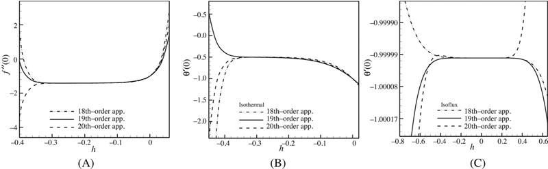
Figure 9.2 h curves for (A) f, (B) θ_isothermal, and (C) θ_isoflux in Re = f_w = Pr = 1, φ = 0.01 and n = 0.

9.1.3. Effects of active parameters

Results are given for the velocity, temperature distribution, wall shear stress and Nusselt number and entropy generation for different nondimensional numbers. Figs. 9.3 and 9.4 are presented to show the effect of the volume fraction of nanoparticles (Cu) on velocity profiles and temperature distribution (A) Power-law temperature, (B) Power-law heat flux, respectively when Pr = 6.2, f_w = 1, Re = 1, n = 2. When the volume of fraction for the nanoparticles increases from 0 to 0.2, all boundary layers thicknesses decrease. This agrees with the physical behavior, when the volume of copper nanoparticles increases the thermal conductivity increases and then the thermal boundary layer thickness decreases. Figs. 9.5 and 9.6 display the behavior of the velocity and the temperature profiles using different nanofluids When Pr = 6.2, φ = 0.1, Re = 1, f_w = 1, n = 2. The tables show that by using different types of nanofluids the values of the velocity and temperature change. When Silver is chosen as the nanoparticle, the maximum amount of all boundary layer thicknesses observed, while minimum amount of those amounts observed by choosing Alumina. (Figs. 9.5 and 9.6). Fig. 9.7 shows variation of skin friction coefficients (–f”(0)) versus (A) Re and (B) f_w for selected values of the nanoparticles volume parameter in the case of Cu–Water. For both suction and injection, it is observed that skin friction increases as φ increases. Also this change occurs when Re or f_w increases. It should be noticed that the changes are more noticeable for higher values of φ when values of Re and f_w are greater. Fig. 9.8 shows variation of Nusselt number for Power-law temperature case (–θ’(0)) versus (A) Re, (B) f_w and (C) n for selected values of the nanoparticles volume parameter in the case of Cu–Water.

Figure 9.3 Effect of nanoparticle volume fraction on velocity profiles when f_w = 1, Re = 1.

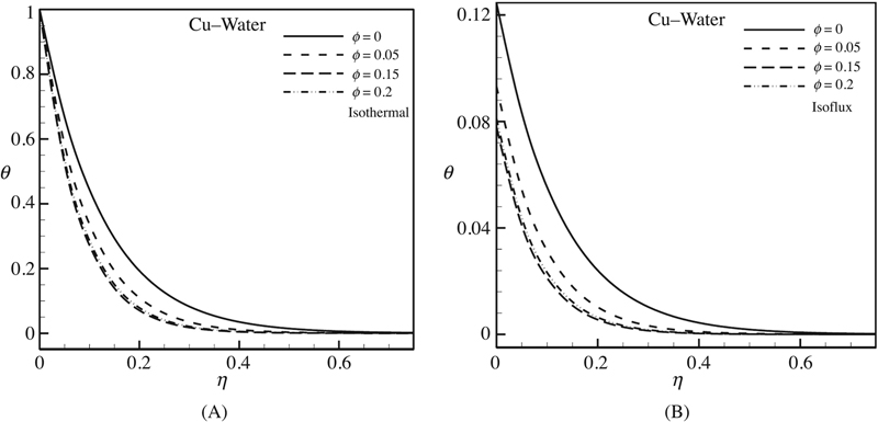
Figure 9.4 Effect of nanoparticle volume fraction on temperature distribution (A) power-law temperature and (B) power-law heat flux when Pr = 6.2, f_w = 1, Re = 1, n = 2.

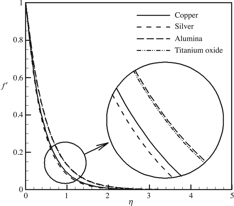
Figure 9.5 Velocity for different types of nanofluids when φ = 0.1, Re = 1, f_w = 1.

Figure 9.6 Temperature profiles (A) power-law temperature and (B) power-law heat flux for different types of nanofluids when Pr = 6.2, φ = 0.1, Re = 1, f_w = 1, n = 2.

Figure 9.7 Effects of the nanoparticle volume fraction φ, Reynolds number, and wall injection/suction parameter on skin friction coefficient when (A) f_w = 1 and (B) Re = 1.

Figure 9.8 Effects of the nanoparticle volume fraction φ, Reynolds number, wall injection/suction parameter, and power of temperature/heat flux distribution on Nusselt number (power-law temperature) when (A) Pr = 6.2, f_w = 1, n = 2, (B) Pr = 6.2, Re = 1, n = 2, and (C) Pr = 6.2, f_w = 1, Re = 1.

It is obvious from Fig. 9.8 that the heat transfer rates increase with the increase of the nanoparticles volume fraction (φ), Re, f_w and n. The change in the Nusselt number is found to be upper for higher values of the parameter φ, and this change are more noticeable with the increase of Re, f_w and n.

Table 9.2 shows the effects of the nanoparticle volume fraction φ for different types of nanofluids on skin friction coefficient when Re = 1, f_w = 1.Tables 9.3 and 9.4 show the effects of the nanoparticle volume fraction φ for different types of nanofluids on Nusselt number for Power-law temperature case, Power-law heat flux case respectively when Pr = 6.2, n = 2, Re = 1, f_w = 1. These tables show that the values of –f”(0), –θ’(0) and 1/θ(0) change with nanofluid changes, that is, we can say that the shear stress and rate of hate transfer change by using different types of nanofluid. This means that the nanofluids will be important in the cooling and heating processes. Choosing Silver as the nanoparticle leads to the maximum amount of skin friction coefficient and rate of hate transfer, while selecting Alumina leads to the minimum amount of those values (Tables 9.2, 9.3 and 9.4). Fig. 9.9 shows the effect of nanoparticle volume fraction on (A) HTI, (B) FFI, (C) S_gen and (D) Be when Pr = 6.2, Re = 1, n = 2, x^* = 0.5, f_w = 1, u₀ = 1m/s, T_∞ = T₀ = 10K, and K = 0.001. Fig. 9.10 shows the effect of different types of nanofluids on (A) HTI, (B) FFI, (C) S_gen and (D) Be when Pr = 6.2, Re = 1, n = 2, φ = 0.1, x^* = 0.5, f_w = 1 u₀ = 1m/s, T_∞ = T₀ = 10K, and K = 0.001. It is observed that, regardless of the boundary condition, increasing percentage of nanoparticles (φ) leads to the increase in the heat transfer irreversibility due to heat transfer in the direction of finite temperature gradients (HTI) and the contribution of fluid friction irreversibility to the total entropy generation (FFI) whereas the increase in HTI is more than increase in FFI. The entropy generation rate (S_gen) reduces while we get farter from the surface of the porous plate and HTI reduction in higher nanoparticles percentages occurs in farter distances. With studying the Bejan number we can see that HTI beats FFI near the surface of porous plate. Adding Alumina nanoparticles leads to the minimum amount of heat loss while the maximum amount of heat loss occurs when we use Silver as the nanoparticles and there will be the same for HTI and FFI. By choosing Silver and Copper as the nanoparticle HTI beats FFI close to the porous plate while selecting Alumina and Titanium Oxide as the nanoparticle cause this fact occurs farter from the porous plate.

Table 9.2

Effects of the nanoparticle volume fraction for different types of nanofluids on skin friction coefficient when Re = 1, f_w = 1

φ	Nanoparticles
φ	Cu	Ag	Al₂O₃	TiO₂
0.05	2.229703	2.298824	2.010783788	2.023135
0.1	2.380028	2.500792	1.9975454	2.019124
0.2	2.483631	2.663553	1.913780762	1.94593

Table 9.3

Effects of the nanoparticle volume fraction for different types of nanofluids on Nusselt number (Power-law temperature) when Pr = 6.2, n = 2, Re = 1, f_w = 1

φ	Nanoparticles
φ	Cu	Ag	Al₂O₃	TiO₂
0.05	10.71299	11.77269	7.741767	8.085111
0.1	12.31904	14.26799	7.201689	7.822867
0.2	12.30637	15.04481	5.630545	6.602276

Table 9.4

Effects of the nanoparticle volume fraction for different types of nanofluids on Nusselt number (Power-law heat flux) when Pr = 6.2, n = 2, Re = 1, f_w = 1

φ	Nanoparticles
φ	Cu	Ag	Al₂O₃	TiO₂
0.05	10.71299	11.77268758	7.741767427	8.085111261
0.1	12.31904	14.26799218	7.201688959	7.822867028
0.2	12.30637	15.04480717	5.630544587	6.60227588

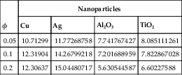
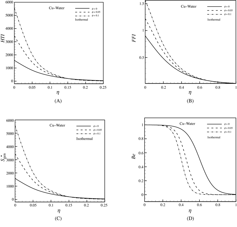
Figure 9.9 Effect of nanoparticle volume fraction on (A) HTI, (B) FFI, and (C) $S_{g e n}^{•}$ $S_{g e n}^{•}$ , and (D) Be When Pr = 6.2, Re = 1, n = 2, x^* = 0.5, f_w = 1 u₀ = 1 m/s, T_∞ = T₀ = 10K, and K = 0.001.

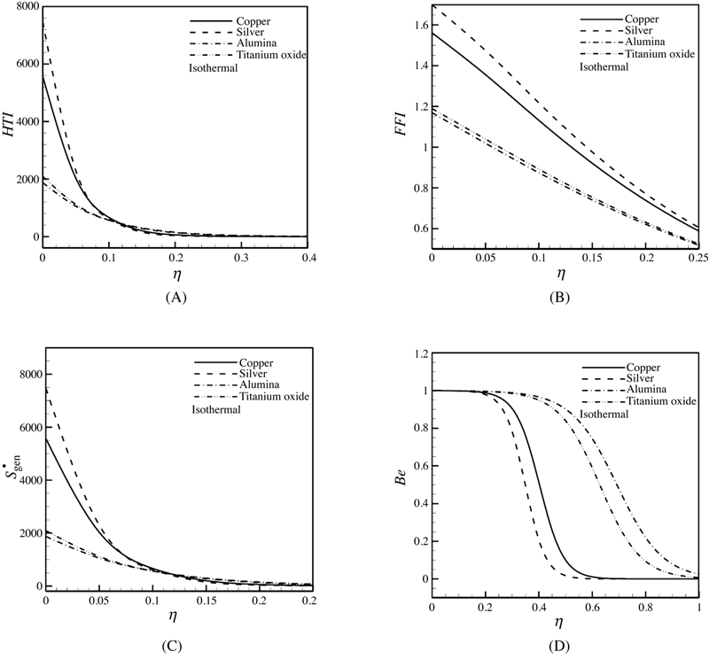
Figure 9.10 Effect of different types of nanofluids on (A) HTI, (B) FFI, (C) $S_{g e n}^{•}$ $S_{g e n}^{•}$ , and (D) Be When Pr = 6.2, Re = 1, n = 2, φ = 0.1, x^* = 0.5, f_w = 1 u₀ = 1 m/s, T_∞ = T₀ = 10K, and K = 0.001.

9.2. Magnetohydrodynamic flow in a permeable channel filled with nanofluid

9.2.1. Problem definition

The laminar two-dimensional stationary nanofluid flow in a semiporous channel made by a long rectangular plate with length of L_x in uniform translation in x* direction and an infinite porous plate is considered. The distance between the two plates is h. We observe a normal velocity q on the porous wall. A uniform magnetic field B is assumed to be applied toward direction y* (Fig. 9.11) [20].

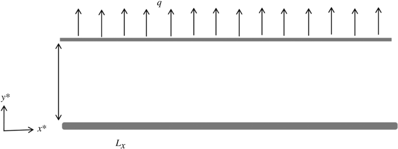
Figure 9.11 Schematic diagram of the system.

In the case of a short circuit to neglect the electrical field and perturbations to the basic normal field and without any gravity forces, the governing equations are:

$\frac{\partial u *}{\partial x *} + \frac{\partial v *}{\partial y *} = 0,$ $\frac{\partial u *}{\partial x *} + \frac{\partial v *}{\partial y *} = 0,$

(9.71)

$u * \frac{\partial u *}{\partial x *} + v * \frac{\partial u *}{\partial y *} = - \frac{1}{ρ_{nf}} \frac{\partial P *}{\partial x *} + \frac{μ_{nf}}{ρ_{nf}} (\frac{\partial^{2} u *}{\partial x *^{2}} + \frac{\partial^{2} u *}{\partial y *^{2}}) - u * \frac{σ_{nf} B^{2}}{ρ_{nf}},$ $u * \frac{\partial u *}{\partial x *} + v * \frac{\partial u *}{\partial y *} = - \frac{1}{ρ_{nf}} \frac{\partial P *}{\partial x *} + \frac{μ_{nf}}{ρ_{nf}} (\frac{\partial^{2} u *}{\partial x *^{2}} + \frac{\partial^{2} u *}{\partial y *^{2}}) - u * \frac{σ_{nf} B^{2}}{ρ_{nf}},$

(9.72)

$u * \frac{\partial v *}{\partial x *} + v * \frac{\partial v *}{\partial y *} = - \frac{1}{ρ_{nf}} \frac{\partial P *}{\partial y *} + \frac{μ_{nf}}{ρ_{nf}} (\frac{\partial^{2} v *}{\partial x *^{2}} + \frac{\partial^{2} v *}{\partial y *^{2}}),$ $u * \frac{\partial v *}{\partial x *} + v * \frac{\partial v *}{\partial y *} = - \frac{1}{ρ_{nf}} \frac{\partial P *}{\partial y *} + \frac{μ_{nf}}{ρ_{nf}} (\frac{\partial^{2} v *}{\partial x *^{2}} + \frac{\partial^{2} v *}{\partial y *^{2}}),$

(9.73)

The appropriate boundary conditions for the velocity are:

$y * = 0 : u * = u_{0} *, v * = 0,$ $y * = 0 : u * = u_{0} *, v * = 0,$

(9.74)

$y * = h : u * = 0, v * = - q,$ $y * = h : u * = 0, v * = - q,$

(9.75)

Calculating a mean velocity U by the relation:

$y * = 0 : u * = u_{0} *, v * = 0,$ $y * = 0 : u * = u_{0} *, v * = 0,$

(9.76)

We consider the following transformations:

$x = \frac{x *}{L_{x}}; y = \frac{y *}{h},$ $x = \frac{x *}{L_{x}}; y = \frac{y *}{h},$

(9.77)

$u = \frac{u *}{U}; v = \frac{v *}{q}, P_{y} = \frac{P *}{ρ_{f} \cdot q^{2}}$ $u = \frac{u *}{U}; v = \frac{v *}{q}, P_{y} = \frac{P *}{ρ_{f} \cdot q^{2}}$

(9.78)

Then, we can consider two dimensionless numbers: the Hartman number Ha for the description of magnetic forces and the Reynolds number Re for dynamic forces:

$H a = B h \sqrt{\frac{σ_{f}}{ρ_{f} . υ_{f}}},$ $H a = B h \sqrt{\frac{σ_{f}}{ρ_{f} . υ_{f}}},$

(9.79)

$R e = \frac{h q}{μ_{nf}} ρ_{nf}$ $R e = \frac{h q}{μ_{nf}} ρ_{nf}$

(9.80)

where the effective density(ρ_nf) is defined as:

$ρ_{nf} = ρ_{f} (1 - φ) + ρ_{s} φ$ $ρ_{nf} = ρ_{f} (1 - φ) + ρ_{s} φ$

(9.81)

Where φ is the solid volume fraction of nanoparticles. The dynamic viscosity, thermal conductivity and effective electrical conductivity of the nanofluid are defined as:

$μ_{nf} = \frac{μ_{f}}{{(1 - φ)}^{2.5}}$ $μ_{nf} = \frac{μ_{f}}{{(1 - φ)}^{2.5}}$

(9.82)

$\frac{k_{n f}}{k_{f}} = \frac{k_{s} + 2 k_{f} - 2 φ (k_{f} - k_{s})}{k_{s} + 2 k_{f} + φ (k_{f} - k_{s})}$ $\frac{k_{n f}}{k_{f}} = \frac{k_{s} + 2 k_{f} - 2 φ (k_{f} - k_{s})}{k_{s} + 2 k_{f} + φ (k_{f} - k_{s})}$

(9.83)

$\frac{σ_{nf}}{σ_{f}} = 1 + \frac{3 (\frac{σ_{s}}{σ_{f}} - 1) φ}{(\frac{σ_{s}}{σ_{f}} + 2) - (\frac{σ_{s}}{σ_{f}} - 1) φ}$ $\frac{σ_{nf}}{σ_{f}} = 1 + \frac{3 (\frac{σ_{s}}{σ_{f}} - 1) φ}{(\frac{σ_{s}}{σ_{f}} + 2) - (\frac{σ_{s}}{σ_{f}} - 1) φ}$

(9.84)

Substituting Eqs. (9.76) and (9.80) into Eqs. (9.71) and (9.73) leads to the dimensionless equations:

$\frac{\partial u}{\partial x} + \frac{\partial v}{\partial y} = 0,$ $\frac{\partial u}{\partial x} + \frac{\partial v}{\partial y} = 0,$

(9.85)

$u \frac{\partial u}{\partial x} + v \frac{\partial u}{\partial y} = - ɛ^{2} \frac{\partial P_{y}}{\partial x} + \frac{μ_{nf}}{ρ_{nf}} \frac{1}{h q} (ɛ^{2} \frac{\partial^{2} u}{\partial x^{2}} + \frac{\partial^{2} u}{\partial y^{2}}) - u \frac{H a^{2}}{Re} \frac{B^{*}}{A^{*}},$ $u \frac{\partial u}{\partial x} + v \frac{\partial u}{\partial y} = - ɛ^{2} \frac{\partial P_{y}}{\partial x} + \frac{μ_{nf}}{ρ_{nf}} \frac{1}{h q} (ɛ^{2} \frac{\partial^{2} u}{\partial x^{2}} + \frac{\partial^{2} u}{\partial y^{2}}) - u \frac{H a^{2}}{Re} \frac{B^{*}}{A^{*}},$

(9.86)

$u \frac{\partial υ}{\partial x} + v \frac{\partial v}{\partial y} = - \frac{\partial P_{y}}{\partial x} + \frac{μ_{nf}}{ρ_{nf}} \frac{1}{h q} (ɛ^{2} \frac{\partial^{2} v}{\partial x^{2}} + \frac{\partial^{2} v}{\partial y^{2}})$ $u \frac{\partial υ}{\partial x} + v \frac{\partial v}{\partial y} = - \frac{\partial P_{y}}{\partial x} + \frac{μ_{nf}}{ρ_{nf}} \frac{1}{h q} (ɛ^{2} \frac{\partial^{2} v}{\partial x^{2}} + \frac{\partial^{2} v}{\partial y^{2}})$

(9.87)

where A^* and B^* are constant parameters:

$A^{*} = (1 - φ) + \frac{ρ_{s}}{ρ_{f}} φ, B * = 1 + \frac{3 (\frac{σ_{s}}{σ_{f}} - 1) φ}{(\frac{σ_{s}}{σ_{f}} + 2) - (\frac{σ_{s}}{σ_{f}} - 1) φ}$ $A^{*} = (1 - φ) + \frac{ρ_{s}}{ρ_{f}} φ, B * = 1 + \frac{3 (\frac{σ_{s}}{σ_{f}} - 1) φ}{(\frac{σ_{s}}{σ_{f}} + 2) - (\frac{σ_{s}}{σ_{f}} - 1) φ}$

(9.88)

Quantity of ɛ is defined as the aspect ratio between distance h and a characteristic length L_x of the slider. This ratio is normally small. Berman’s similarity transformation is used to be free from the aspect ratio of ɛ:

$v = - V (y); u = \frac{u *}{U} = u_{0} U (y) + x \frac{d V}{d y}$ $v = - V (y); u = \frac{u *}{U} = u_{0} U (y) + x \frac{d V}{d y}$

(9.89)

Introducing Eq. (9.89) in the second momentum equation (9.87) shows that quantity ∂P_y/∂y does not depend on the longitudinal variable x. With the first momentum equation, we also observe that ∂²P_y/∂x² is independent of x. We omit asterisks for simplicity. Then a separation of variables leads to:

$V^{' 2} - V V^{''} - \frac{1}{R e} \frac{1}{A^{*} {(1 - φ)}^{2.5}} V^{'''} + \frac{H a^{2}}{R e} \frac{B^{*}}{A^{*}} V^{'} = ɛ^{2} \frac{\partial^{2} P_{y}}{\partial x^{2}} = ɛ^{2} \frac{1}{x} \frac{\partial P_{y}}{\partial x},$ $V^{' 2} - V V^{''} - \frac{1}{R e} \frac{1}{A^{*} {(1 - φ)}^{2.5}} V^{'''} + \frac{H a^{2}}{R e} \frac{B^{*}}{A^{*}} V^{'} = ɛ^{2} \frac{\partial^{2} P_{y}}{\partial x^{2}} = ɛ^{2} \frac{1}{x} \frac{\partial P_{y}}{\partial x},$

(9.90)

$U V^{'} - V U^{'} = \frac{1}{R e} \frac{1}{A^{*} {(1 - φ)}^{2.5}} [U^{''} - H a^{2} B^{*} {(1 - φ)}^{2.5} U]$ $U V^{'} - V U^{'} = \frac{1}{R e} \frac{1}{A^{*} {(1 - φ)}^{2.5}} [U^{''} - H a^{2} B^{*} {(1 - φ)}^{2.5} U]$

(9.91)

The right-hand side of Eq. (9.90) is constant. So, we derive this equation with respect to x. This gives:

$V^{I V} = H a^{2} B^{*} {(1 - φ)}^{2.5} V^{''} + Re A^{*} {(1 - φ)}^{2.5} [V^{'} V^{''} - V V^{'''}],$ $V^{I V} = H a^{2} B^{*} {(1 - φ)}^{2.5} V^{''} + Re A^{*} {(1 - φ)}^{2.5} [V^{'} V^{''} - V V^{'''}],$

(9.92)

Where primes denote differentiation with respect to y and asterisks have been omitted for simplicity. The dynamic boundary conditions are:

$y = 0 : U = 1; V = 0; V^{'} = 0,$ $y = 0 : U = 1; V = 0; V^{'} = 0,$

(9.93)

$y = 1 : U = 0; V = 1; V^{'} = 0 .$ $y = 1 : U = 0; V = 1; V^{'} = 0 .$

(9.94)

9.2.2. Semi analytical method

9.2.2.1. Basic idea of OHAM

Following differential equation is considered:

$L (u (t)) + N (u (t)) + g (t) = 0, B (u) = 0,$ $L (u (t)) + N (u (t)) + g (t) = 0, B (u) = 0,$

(9.95)

where L is a linear operator, τ is an independent variable, u(t) is an unknown function, g(t) is a known function, N(u(t)) is a nonlinear operator and B is a boundary operator. By means of OHAM one first constructs a set of equations:

$\begin{array}{l} (1 - p) [L (φ (τ, p)) + g (τ)] - H (p) [L (φ (τ, p)) + g (τ) + N (φ (τ, p))] = 0 \\ B (φ (τ, p)) = 0, \end{array}$ $\begin{array}{l} (1 - p) [L (φ (τ, p)) + g (τ)] - H (p) [L (φ (τ, p)) + g (τ) + N (φ (τ, p))] = 0 \\ B (φ (τ, p)) = 0, \end{array}$

(9.96)

where p ∈ [0.1] is an embedding parameter, H(p) denotes a nonzero auxiliary function for p ≠ 0 and H(0) = 0, φ(τ, p) is an unknown function. Obviously, when p = 0 and p = 1, it holds that:

$φ (τ, 0) = u_{0} (τ), \cdot φ (τ, 1) = u (τ)$ $φ (τ, 0) = u_{0} (τ), \cdot φ (τ, 1) = u (τ)$

(9.97)

Thus, as p increases from 0 to 1, the solution φ(τ, p) varies from u₀(τ) to the solution u(τ), where u₀(τ) is obtained from Eq. (9.96) for p = 0:

$L (u_{0} (τ)) + g (τ) = 0, \cdot B (u_{0}) = 0 .$ $L (u_{0} (τ)) + g (τ) = 0, \cdot B (u_{0}) = 0 .$

(9.98)

We choose the auxiliary function H(p) in the form:

$H (p) = p C_{1} + p_{2} C_{2} + .. .$ $H (p) = p C_{1} + p_{2} C_{2} + .. .$

(9.99)

Where C₁, C₂, ... are constants which can be determined later.

Expanding φ(τ, p) in a series with respect to p, one has:

$φ (τ, p, C_{i}) = u_{0} (τ) + \sum_{k \geq 1} u_{k} (τ, C_{i}) p_{k}, \cdot i = 1,2,.. .$ $φ (τ, p, C_{i}) = u_{0} (τ) + \sum_{k \geq 1} u_{k} (τ, C_{i}) p_{k}, \cdot i = 1,2,.. .$

(9.100)

Substituting Eq. (9.100) into Eq. (9.86), collecting the same powers of p, and equating each coefficient of p to zero, we obtain set of differential equation with boundary conditions. Solving differential equations by boundary conditions u₀(τ), u₁(τ, C₁), u₂(τ, C₂),... are obtained. Generally speaking, the solution of Eq. (9.95) can be determined approximately in the form:

${\tilde{u}}^{(m)} = u_{0} (τ) + \sum_{k = 1}^{m} u_{k} (τ, C_{i})$ ${\tilde{u}}^{(m)} = u_{0} (τ) + \sum_{k = 1}^{m} u_{k} (τ, C_{i})$

(9.101)

Note that the last coefficient C_m can be function of τ. Substituting Eq. (9.98) into Eq. (9.95), there results the following residual:

$R (τ, C_{i}) = L ({\tilde{u}}^{(m)} (τ, C_{i})) + g (τ) + N ({\tilde{u}}^{(m)} (τ, C_{i})) .$ $R (τ, C_{i}) = L ({\tilde{u}}^{(m)} (τ, C_{i})) + g (τ) + N ({\tilde{u}}^{(m)} (τ, C_{i})) .$

(9.102)

If Re(τ, C_i) = 0 then ũ^(m)(τ, C_i) happens to be the exact solution. Generally such a case will not arise for nonlinear problems, but we can minimize the functional by Galerkin method (GM):

$w_{i} = \frac{\partial R e (τ, C_{1}, C_{2}, ..., C_{m})}{\partial C_{i}}, i = 1,2,..., m,$ $w_{i} = \frac{\partial R e (τ, C_{1}, C_{2}, ..., C_{m})}{\partial C_{i}}, i = 1,2,..., m,$

(9.103)

The unknown constants C_i(i = 1, 2,...,m) can be identified from the conditions:

$J (C_{1}, C_{2}) = \int_{a}^{b} w_{i} . R e (τ, C_{1}, C_{2}, ..., C_{m}) d τ = 0,$ $J (C_{1}, C_{2}) = \int_{a}^{b} w_{i} . R e (τ, C_{1}, C_{2}, ..., C_{m}) d τ = 0,$

(9.104)

where a and b are two values, depending on the given problem. With these constants, the approximate solution (of order m) [Eq. (9.101)] is well determined. It can be observed that the method proposed in this work generalizes these two methods using the special (more general) auxiliary function H(p).

9.2.2.2. Application of OHAM

In this section, OHAM is applied to nonlinear ordinary differential Eqs. (9.91) and (9.92). According to the OHAM, we have:

$\begin{array}{l} V^{I V} = H a^{2} B^{*} {(1 - φ)}^{2.5} V^{''} + R e A^{*} {(1 - φ)}^{2.5} [V^{'} V^{''} - V V^{'''}], \\ U V^{'} - V U^{'} = \frac{1}{R e} \frac{1}{A^{*} {(1 - φ)}^{2.5}} [U^{''} - H a^{2} B^{*} {(1 - φ)}^{2.5} U] \cdot \end{array}$ $\begin{array}{l} V^{I V} = H a^{2} B^{*} {(1 - φ)}^{2.5} V^{''} + R e A^{*} {(1 - φ)}^{2.5} [V^{'} V^{''} - V V^{'''}], \\ U V^{'} - V U^{'} = \frac{1}{R e} \frac{1}{A^{*} {(1 - φ)}^{2.5}} [U^{''} - H a^{2} B^{*} {(1 - φ)}^{2.5} U] \cdot \end{array}$

(9.105)

We consider V, U, H₁(p) and H₂(p) as following:

$\begin{array}{l} V = V_{0} + p V_{1} + p^{2} V_{2}, \cdot U = U_{0} + p U_{1} + p^{2} U_{2}, \\ H_{1} (p) = p C_{11} + p^{2} C_{12}, H_{2} (p) = p C_{21} + p^{2} C_{22} \end{array}$ $\begin{array}{l} V = V_{0} + p V_{1} + p^{2} V_{2}, \cdot U = U_{0} + p U_{1} + p^{2} U_{2}, \\ H_{1} (p) = p C_{11} + p^{2} C_{12}, H_{2} (p) = p C_{21} + p^{2} C_{22} \end{array}$

(9.106)

Substituting V, U, H₁(p) and H₂(p) from Eq. (9.106) into Eq. (9.105) and some simplification and rearranging based on powers of p-terms, we have:

$\begin{array}{l} p^{0} : V^{I V} = 0, \\ U^{''} = 0, \\ V_{0} (0) = 0, V_{0}^{'} (0) = 0, V_{0} (1) = 1, V_{0}^{'} (1) = 0 \\ U_{0} (0) = 1, U_{0} (1) = 0 \end{array}$ $\begin{array}{l} p^{0} : V^{I V} = 0, \\ U^{''} = 0, \\ V_{0} (0) = 0, V_{0}^{'} (0) = 0, V_{0} (1) = 1, V_{0}^{'} (1) = 0 \\ U_{0} (0) = 1, U_{0} (1) = 0 \end{array}$

(9.107)

$\begin{array}{l} p^{1} : \\ \begin{array}{l} {V_{1}}^{I V} + C_{11} {V_{0}}^{I V} - C_{11} Re A^{*} {(1 - φ)}^{2.5} {V_{0}}^{''} {V_{0}}^{'} + C_{11} Re A^{*} {(1 - φ)}^{2.5} {V_{0}}^{'''} V_{0} \\ - C_{11} H a^{2} B^{*} {(1 - φ)}^{2.5} {V_{0}}^{''} - {V_{0}}^{I V} = 0, \end{array} \\ \begin{array}{l} U_{1}^{''} - C_{21} Re A^{*} {(1 - φ)}^{2.5} V_{0}^{'} U_{0} + C_{22} U_{0}^{''} - U_{0}^{''} + C_{21} Re A^{*} {(1 - φ)}^{2.5} U_{0}^{'} V_{0} \\ - C_{21} H a^{2} B^{*} {(1 - φ)}^{2.5} U_{0} = 0 \end{array} \\ V_{1} (0) = 0, V_{1}^{'} (0) = 0, V_{1} (1) = 0, V_{1}^{'} (1) = 0 \\ \begin{array}{l} U_{1} (0) = 0, U_{1} (1) = 0 \\ ⋮ \end{array} \end{array}$ $\begin{array}{l} p^{1} : \\ \begin{array}{l} {V_{1}}^{I V} + C_{11} {V_{0}}^{I V} - C_{11} Re A^{*} {(1 - φ)}^{2.5} {V_{0}}^{''} {V_{0}}^{'} + C_{11} Re A^{*} {(1 - φ)}^{2.5} {V_{0}}^{'''} V_{0} \\ - C_{11} H a^{2} B^{*} {(1 - φ)}^{2.5} {V_{0}}^{''} - {V_{0}}^{I V} = 0, \end{array} \\ \begin{array}{l} U_{1}^{''} - C_{21} Re A^{*} {(1 - φ)}^{2.5} V_{0}^{'} U_{0} + C_{22} U_{0}^{''} - U_{0}^{''} + C_{21} Re A^{*} {(1 - φ)}^{2.5} U_{0}^{'} V_{0} \\ - C_{21} H a^{2} B^{*} {(1 - φ)}^{2.5} U_{0} = 0 \end{array} \\ V_{1} (0) = 0, V_{1}^{'} (0) = 0, V_{1} (1) = 0, V_{1}^{'} (1) = 0 \\ \begin{array}{l} U_{1} (0) = 0, U_{1} (1) = 0 \\ ⋮ \end{array} \end{array}$

(9.108)

Solving Eqs. (9.107) and (9.108) with boundary conditions:

$\begin{array}{l} V_{0} (y) = - 2 y^{3} + 3 y^{2}, \\ U_{0} (y) = - y + 1, \end{array}$ $\begin{array}{l} V_{0} (y) = - 2 y^{3} + 3 y^{2}, \\ U_{0} (y) = - y + 1, \end{array}$

(9.109)

$\begin{array}{l} V_{1} (y) = C_{11} (0.05714285714 Re A^{*} {(1 - φ)}^{2.5} y^{7} - 0.2 y^{6} - 0.1 H a^{2} B^{*} {(1 - φ)}^{2.5} y^{5} \\ + 0.25 H a^{2} B^{*} {(1 - φ)}^{2.5} y^{4} - 0.3857142857 Re A^{*} {(1 - φ)}^{2.5} y^{3} \\ - 0.2 H a^{2} B^{*} {(1 - φ)}^{2.5} y^{3} + (0.22855714286 Re A^{*} {(1 - φ)}^{2.5} + 0.05) y^{2}), \\ U (y) = C_{21} (0.2 Re y^{5} - 0.75 Re A^{*} {(1 - φ)}^{2.5} y^{4} + Re A^{*} {(1 - φ)}^{2.5} y^{3} \\ - 0.1667 H a^{2} B^{*} {(1 - φ)}^{2.5} y^{3} + 0.5 H a^{2} B^{*} {(1 - φ)}^{2.5} y^{2} \\ - 0.45 Re A^{*} {(1 - φ)}^{2.5} y - 0.3333 H a^{2} B^{*} {(1 - φ)}^{2.5} y) \end{array}$ $\begin{array}{l} V_{1} (y) = C_{11} (0.05714285714 Re A^{*} {(1 - φ)}^{2.5} y^{7} - 0.2 y^{6} - 0.1 H a^{2} B^{*} {(1 - φ)}^{2.5} y^{5} \\ + 0.25 H a^{2} B^{*} {(1 - φ)}^{2.5} y^{4} - 0.3857142857 Re A^{*} {(1 - φ)}^{2.5} y^{3} \\ - 0.2 H a^{2} B^{*} {(1 - φ)}^{2.5} y^{3} + (0.22855714286 Re A^{*} {(1 - φ)}^{2.5} + 0.05) y^{2}), \\ U (y) = C_{21} (0.2 Re y^{5} - 0.75 Re A^{*} {(1 - φ)}^{2.5} y^{4} + Re A^{*} {(1 - φ)}^{2.5} y^{3} \\ - 0.1667 H a^{2} B^{*} {(1 - φ)}^{2.5} y^{3} + 0.5 H a^{2} B^{*} {(1 - φ)}^{2.5} y^{2} \\ - 0.45 Re A^{*} {(1 - φ)}^{2.5} y - 0.3333 H a^{2} B^{*} {(1 - φ)}^{2.5} y) \end{array}$

(9.110)

The terms of V₂(y) and U₂(y) are too large that mentioned graphically. Therefore, final expression for V(y) and U(y) is:

$\begin{array}{l} V (y) = V_{0} (y) + V_{1} (y) + V_{2} (y) \\ U (y) = U_{0} (y) + U_{1} (y) + U_{2} (y) \end{array}$ $\begin{array}{l} V (y) = V_{0} (y) + V_{1} (y) + V_{2} (y) \\ U (y) = U_{0} (y) + U_{1} (y) + U_{2} (y) \end{array}$

(9.111)

By Substituting V(y) and U(y) into Eq. (9.105), R₁(η, C₁₁, C₁₂) and R₂(η, C₂₁, C₂₂) are obtained then J₁ and J₂ are obtained in the flowing manner:

$J (C_{11}, C_{12}) = \int_{a}^{b} w_{i} . R_{1} d τ = 0,$ $J (C_{11}, C_{12}) = \int_{a}^{b} w_{i} . R_{1} d τ = 0,$

(9.112)

$J (C_{21}, C_{22}) = \int_{a}^{b} w_{i} . R_{2} d τ = 0 .$ $J (C_{21}, C_{22}) = \int_{a}^{b} w_{i} . R_{2} d τ = 0 .$

(9.113)

The constants C₁₁, C₁₂, C₂₁, and C₂₂ obtain from Eqs. (9.112) and (9.113). By substituting these constants into Eq. (9.111), an expression for V(y) and U(y) is obtained.

9.2.3. Effects of active parameters

In the present laminar nanofluid flow in a permeable channel in the presence of uniform magnetic field is studied (Fig. 9.11). Optimal Homotopy Asymptotic Method (using Galerkin method to minimize the residual) is used in order to solve this problem.

Fig. 9.12 shows the effects of various values of Hartmann number on V(y) and U(y). Generally, when the magnetic field is imposed on the enclosure, the velocity field suppressed owing to the retarding effect of the Lorenz force. For low Reynolds number, as Hartmann number increases V(y) decreases for y > y_m but opposite trend is observed for y < y_m, y_m is a meeting point that all curves joint together at this point. When Reynolds number increases this meeting point shifts to the solid wall and it can be seen that V(y) decreases with increase of Hartmann number. As Hartmann number increases U(y) decreases for all values of Reynolds number. Besides, this figure shows that this change is more pronounced for low Reynolds numbers.

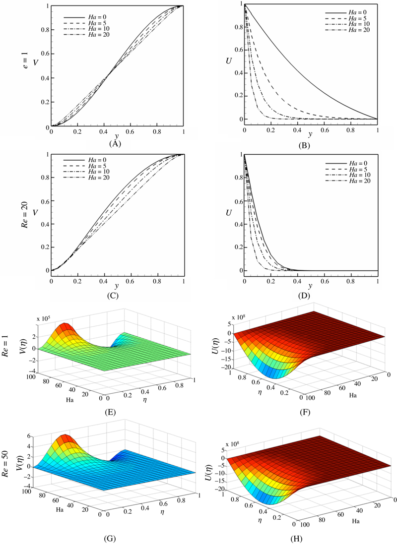
Figure 9.12 Effect of various values of Hartmann numbers (Ha) on V(y) and U(y), when φ = 0.06.

Fig. 9.13 shows the effects of various values of Reynolds numbers (Re) on V(y) and U(y). It is worth to mention that the Reynolds number indicates the relative significance of the inertia effect compared to the viscous effect. Thus, velocity profile decreases as Re increases and in turn increasing Re leads to increase in the magnitude of the skin friction coefficient. With increasing Reynolds number, V(y) and U(y) increase. These effects become less at higher Hartmann numbers because of retarding flow owing to Lorenz forces. Also it shows that increasing Hartmann number leads to increasing the curve of velocity profile.

Figure 9.13 Effects of various values of Reynolds numbers (Re) on V(y) and U(y), when φ = 0.06.

..................Content has been hidden....................

You can't read the all page of ebook, please click here login for view all page.

Table of Contents for Chapter 9: Nanofluid Flow and Heat Transfer in Porous Media

Create new playlist

Sign In

Sign Up

Abstract

Keywords

9.1. Nanofluid heat Transfer over a permeable stretching wall in a porous medium

9.1.1. Problem definition

9.1.2. Semi analytical method

9.1.2.1. Basic idea of HAM

9.1.2.2. Application of HAM

9.1.3. Effects of active parameters

9.2. Magnetohydrodynamic flow in a permeable channel filled with nanofluid

9.2.1. Problem definition

9.2.2. Semi analytical method

9.2.2.1. Basic idea of OHAM

9.2.2.2. Application of OHAM

9.2.3. Effects of active parameters

Table of Contents for
Chapter 9: Nanofluid Flow and Heat Transfer in Porous Media