
3.5. Nanofluid flow and heat transfer between parallel plates considering Brownian motion using DTM
3.5.1. Problem definition
We consider the flow and heat transfer analysis in the unsteady two-dimensional squeezing flow of an incompressible nanofluid between the infinite parallel plates (Fig. 3.36). The two plates are placed at  (
( is distant of plate at t = 0 and α is squeezed parameter). For α > 0, the two plates are squeezed until they touch t = 1/α and for α < 0, the two plates are separated. The viscous dissipation effect, the generation of heat due to fraction caused by shear in the flow, is neglected. Further the symmetric nature of the flow is adopted Ref. [10]. It is also assumed that the time variable magnetic field
  is applied, where
  is unit vectors in the Cartesian coordinate system. The electric current J and the electromagnetic force F are defined by
  and
and  , respectively. Also a heat source (Q = Q0/(1 − αt)) is applied between two plates.
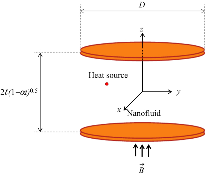
Figure 3.36 Geometry of problem.
The nanofluid is a two-component mixture with the following assumptions: incompressible, no-chemical reaction, negligible radiative heat transfer, and nanosolid-particles and the base fluid are in thermal equilibrium and no slip occurs between them.
The governing equations for conservative momentum and energy in unsteady two-dimensional flow of a nanofluid fluid are according to Ref. [11]:
 (3.91)
 (3.92)
 (3.93)
 (3.94)
Here u and  are the velocities in the x and y directions respectively, T is the temperature,
P is the pressure, effective density (ρnf), the effective heat capacity  and electrical conductivity (σnf) of the nanofluid are defined as:
 (3.95)
 (3.96)
 (3.97)
The relevant boundary conditions are:
 (3.98)
We introduce these parameters:
 (3.99)
Substituting the aforementioned variables into Eqs. (3.92) and (3.93), and then eliminating the pressure gradient from the resulting equations give:
 (3.101)
Here A1, A2, A3, A4, and A5 are dimensionless constants given by:
 (3.102)
With these boundary conditions:
 (3.103)
where S is the squeeze number, Pr is the Prandtl number, Ha is the Hartmann number, and  is the heat source parameter, which are defined as:
 (3.104)
Physical quantities of interest are the skin fraction coefficient and Nusselt number, which are defined as:
 (3.105)
In terms of (3.105), we obtain
 (3.106)
3.5.2. Semianalytical method
3.5.2.1. Basic idea of DTM
Basic definitions and operations of differential transformation are introduced as follows. Differential transformation of the function f(η) is defined as follows:
 (3.107)
In Eq. (3.107), f(η) is the original function and F(k) is the transformed function, which is called the T-function [it is also called the spectrum of the f(η) at η = η0, in the k domain]. The differential inverse transformation of F(k) is defined as:
 (3.108)
 (3.109)
Eq. (3.109) implies that the concept of the differential transformation is derived from Taylor’s series expansion, but the method does not evaluate the derivatives symbolically. However, relative derivatives are calculated by an iterative procedure that is described by the transformed equations of the original functions. From the definitions of Eqs. (3.107) and (3.108), it is easily proven that the transformed functions comply with the basic mathematical operations shown further. In real applications, the function f(η) in Eq. (3.109) is expressed by a finite series and can be written as:
 (3.110)
Eq. (3.110) implies that  is negligibly small, where N is series size. Theorems to be used in the transformation procedure, which can be evaluated from Eqs. (3.107) and (3.108), are given in Table 3.8.
Table 3.8
Some of the basic operations of differential transformation method (DTM)
| Original function | Transformed function |
| f(η) = αg(η) ± βh(η) | F[k] = αG[k] ± βH[k] |
|
|
| f(η) = g(η)h(η) |
|
| f(τ) = sin(ϖη + α) |
|
| f(τ) = cos(ϖη + α) |
|
| f(η) = eλη |

|
| F(η) = (1 + η)m |
|
| f(η) = ηm |
|

3.5.2.2. Application of DTM
Now differential transformation method (DTM) has been applied into governing equations [Eqs. (3.100) and (3.101)]. Taking the differential transforms of equations Eqs. (3.100) and (3.101) with respect to χ and considering H = 1 gives:
 (3.111)
 (3.113)
where F[k] and Θ[k] are the differential transforms of f(η), θ(η) and a1, a2, and a3 are constants, which can be obtained through boundary condition. This problem can be solved as followed:
 (3.115)
 (3.116)
This process is continuous. By substituting Eqs. (3.115) and (3.116) into the main Eq. (3.110) based on DTM, it can be obtained that the closed form of the solutions is:
 (3.117)
 (3.118)
by substituting the boundary condition from Eq. (3.103) into Eqs. (3.117) and (3.118) in point η = 1, the values of a1, a2, and a3 can be obtained. By substituting obtained a1, a2, and a3 into Eqs. (3.117) and (3.118), the expression of F(η) and Θ(η) can be obtained.
3.5.3. Effects of active parameters
In this study, unsteady flow between parallel plates in the presence of variable magnetic field is investigated analytically using DTM. The type of nanoparticle is a key factor for heat transfer enhancement. Tables 3.9 and 3.10 show a comparison between two different types of nanoparticles, which enables selection of a nanoparticle that leads to a higher enhancement for this problem. It is also found that choosing CuO as the nanoparticle leads a greater amount of the skin friction coefficient and Nusselt number. So we select CuO-water as a nanofluid. The influences of the squeeze number, Hartmann number, heat source, and the nanofluid volume fraction on the flow and heat transfer characteristics that are studied. Fig. 3.37 shows the effect of nanofluid volume fraction on the skin friction coefficient and Nusselt number. As the nanofluid volume fraction increases, Nusselt number increases, while skin friction coefficient decreases.
Table 3.9
Comparison of the skin friction coefficient between Al2O3–water and CuO–water at ɸ = 0.04 and Pr = 6.2
| S | Ha | Cf | |
| CuO | Al2O3 | ||
| 1 | 0 | 3.779263 | 3.629287 |
| 1 | 8 | 8.809621 | 8.676915 |
| 10 | 0 | 7.23826 | 6.897281 |
| 10 | 8 | 10.61304 | 10.33316 |

Table 3.10
Comparison of the Nusselt number between Al2O3–water and CuO–water at ɸ = 0.04 and Pr = 6.2
| Hs | S | Ha | Nu | |
| CuO | Al2O3 | |||
| –1 | 1 | 0 | 0.717776 | 0.632233 |
| –1 | 1 | 8 | 0.78598 | 0.700244 |
| –1 | 10 | 0 | 0.291036 | 0.243075 |
| –1 | 10 | 8 | 0.348638 | 0.293618 |
| –10 | 10 | 8 | 3.532066 | 2.130418 |


Figure 3.37 Effect of volume fraction of nanofluid on the (A) skin friction coefficient and (B) Nusselt number when S = 1, Hs = −1, and Pr = 6.2 (CuO–water).
Fig. 3.38 shows the effect of the squeeze number on the velocity and temperature profiles. It is important to note that the squeeze number (S) describes the movement of the plates (S > 0 corresponds to the plates moving apart, while S < 0 corresponds to the plates moving together the so-called squeezing flow). Vertical velocity decreases with an increase in squeeze number, while horizontal velocity has a different behavior. It means that the horizontal velocity decreases with an increase in S when η < 0.5, while the opposite trend is observed for η > 0.5. Thermal boundary layer thickness increases with an increase in squeeze number. Effect of the Hartmann number on the velocity and temperature profiles is shown in Fig. 3.39. Effects of Hartmann number on the velocity profiles are similar to that of the squeeze number. However, an increase in Hartmann number leads to a decrease in thermal boundary layer thickness.
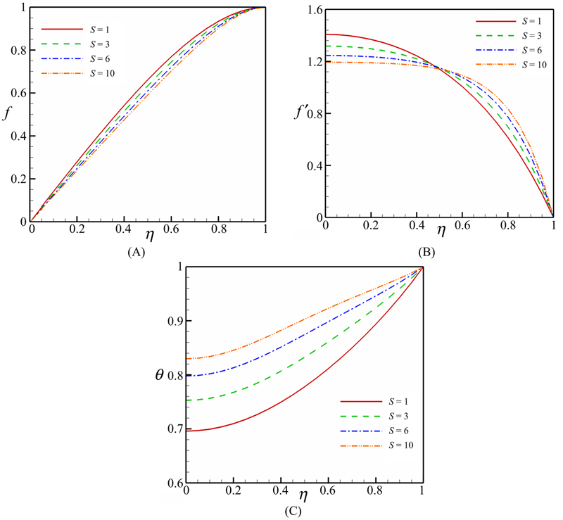
Figure 3.38 Effect of the squeeze number on (A–B) velocity and (C) temperature profiles when Ha = 1, Hs = −1, and Pr = 6.2 (CuO–water).
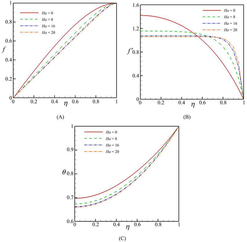
Figure 3.39 Effect of the Hartmann number on (A–B) velocity and (C) temperature profiles when S = 1, Hs = −1, and Pr = 6.2 (CuO–water).
Fig. 3.40 depicts the effects of Hartmann number and squeeze number on the skin friction coefficient and Nusselt number. This figure shows that the Hartmann number has a direct relationship with both the skin friction coefficient and Nusselt number. However, the squeeze number has a direct relationship with the skin friction coefficient and a reverse relationship with the Nusselt number. Effects of the heat source parameter on the temperature profile and Nusselt number is shown in Fig. 3.41. As the heat source parameter increases, temperature boundary layer thickness decreases and in turn the Nusselt number increases.

Figure 3.40 Effects of Hartmann number and squeeze number on the (A) skin friction coefficient and (B) Nusselt number when ɸ = 0.04, Hs = −1, and Pr = 6.2 (CuO–water).
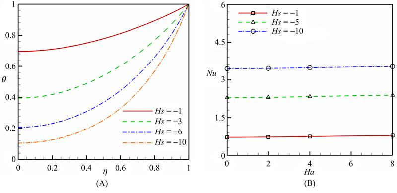
Figure 3.41 Effects of heat source parameter on the (A) temperature profile and (B) Nusselt number when ɸ = 0.04, Hs = −1, and Pr = 6.2 (CuO–water).
3.6. Effect of Lorentz forces on forced convection nanofluid flow over a stretched surface
3.6.1. Problem definition and mathematical model
3.6.1.1. Problem definition
Consider the steady, two-dimensional flow of a nanofluid near the stagnation point on a stretching sheet saturated in the presence of transverse magnetic field as shown in Fig. 3.42 [12]. The stretching velocity  and the free stream velocity U∞(x) are assumed to vary proportionally to the distance x from the stagnation point, that is,
  and U∞(x) = bx, where a and b are constants with a > 0 and b ≥ 0. It is also assumed that the surface of the sheet is subjected to a prescribed temperature
  , where T∞ is the ambient fluid temperature and c and n are constants with c > 0 (heated surface). Further, a uniform magnetic field of strength B0 is assumed to be applied in the positive y-direction normal to the stretching sheet. The magnetic Reynolds number is assumed to be small, and thus the induced magnetic field is negligible. Also the thermal radiation effect is considered in this problem.

Figure 3.42 Figure of geometery.
The nanofluid is a two-component mixture with the following assumptions: incompressible, no-chemical reaction, negligible radiative heat transfer, nanosolid particles and the base fluid are in thermal equilibrium, and no slip occurs between them. Under these assumptions the governing equations are:
 (3.119)
 (3.120)
 (3.121)
Subject to the boundary conditions
 (3.122)
where u and are the velocity components along the x and y axes, respectively and T is fluid temperature. The radiation heat flux qr is considered according to Rosseland approximation, such that  where σe, βR are the Stefan–Boltzmann constant and the mean absorption coefficient, respectively. The fluid-phase temperature differences within the flow are assumed to be sufficiently small, such that T 4 may be expressed as a linear function of temperature. This is done by expanding T 4 in a Taylor series about the temperature Tc and neglecting the higher-order terms to yield,
  .
.
where σe, βR are the Stefan–Boltzmann constant and the mean absorption coefficient, respectively. The fluid-phase temperature differences within the flow are assumed to be sufficiently small, such that T 4 may be expressed as a linear function of temperature. This is done by expanding T 4 in a Taylor series about the temperature Tc and neglecting the higher-order terms to yield, The effective density ρnf, the heat capacitance , and electrical conductivity (σnf) of the nanofluid are given as:
 (3.125)
 (3.126)
(3.127)The continuity Eq. (3.119) is satisfied by introducing a stream function ψ, such that
 (3.128)
The momentum and energy equations can be transformed into the corresponding ordinary differential equations by the following transformation:
 (3.129)
The transformed ordinary differential equations are:
 (3.130)
 (3.131)
subject to the boundary conditions (3.122), which become
 (3.132)
Here prime denote differentiation with respect to η, λ = b/a is the velocity ratio parameter,  , Pr is the Prandtl number,
  is the magnetic parameter and
  is Radiation parameter. Also A1, A2, A3, A4, and A5 are parameters having the following form:
 (3.133)
The skin friction coefficient and the local Nusselt number can be expressed as:
 (3.134)
3.6.1.2. Numerical method
Before employing the Runge–Kutta integration scheme, first we reduce the governing differential equations into a set of first-order ODEs.
Let x1 = η, x2 = f, x3 = f′, x4 = f″, x5 = θ, and x6 = θ′. We obtain the following system:
 (3.135)
and the corresponding initial conditions are
 (3.136)
The earlier nonlinear coupled ODEs along with initial conditions are solved using fourth-order Runge–Kutta integration technique. Suitable values of the unknown initial conditions
u1 and u2 are approximated through Newton’s method until the boundary conditions at f′(∞)→λ, θ(∞)→0 are satisfied. The computations have been performed using MAPLE. The maximum value of η = ∞, to each group of parameters is determined when the values of unknown boundary conditions at x = 0 do not change to a successful loop with error less than 10−6.
3.6.2. Effects of active parameters
The governing ordinary differential equations have been solved numerically for some values of the governing parameters: radiation parameter, magnetic parameter, nanoparticle volume fraction, velocity ratio parameter, and temperature index parameter using the fourth-order Runge–Kutta integration scheme featuring a shooting technique.
Fig. 3.43 shows the effect of magnetic parameter on the velocity and temperature profiles. The magnetic parameter represents the importance of magnetic field on the flow. The presence of transverse magnetic field sets in Lorentz force, which results in a retarding force on the velocity field. Therefore, as the magnetic parameter increases, so does the retarding force and hence the thickness of the boundary layer decreases. As the magnetic parameter increases, velocity boundary layer thickness decreases, while thermal boundary layer thickness increases. Fig. 3.44 depicts the effect of the velocity ratio parameter on the velocity and temperature profiles. When λ < 1, the flow has an inverted boundary layer structure, which results from the fact that when b/a < 1, the stretching velocity ax of the surface exceeds the velocity bx of the external stream. Velocity boundary layer thickness increases with an increase in the velocity ratio parameter, while the opposite trend is observed for thermal boundary layer thickness.
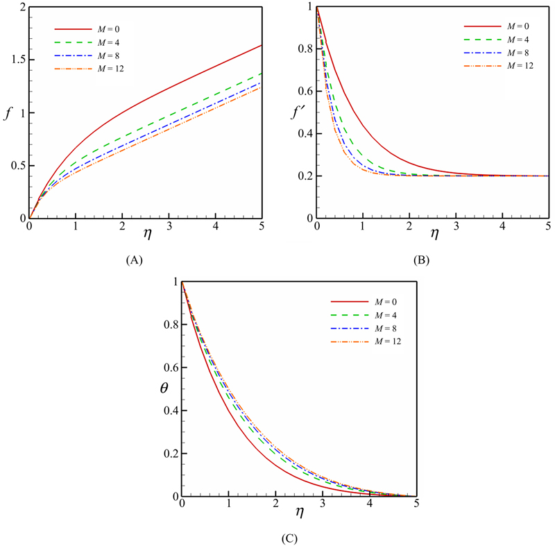
Figure 3.43 Effect of magnetic parameter on (A–B) velocity and (C) temperature profiles when Pr = 6.2, ɸ = 0.04, λ = 0.2, Rd = 5, and n = 1.

Figure 3.44 Effect of velocity ratio parameter on the (A–B) velocity and (C) temperature profiles when Pr = 6.2, ɸ = 0.04, M = 1, and Rd = 5, and n = 1.
Effects of velocity ratio parameter and magnetic parameter on the skin friction coefficient and Nusselt number are shown in Fig. 3.45. Skin friction coefficient increases with an increase in magnetic parameter, but decreases with an increase in velocity ratio parameter. Nusselt number has a direct relationship with the velocity ratio parameter, while it has a reverse relationship with magnetic parameter. Fig. 3.46 shows the effect of radiation parameter on the temperature profile and Nusselt number. Thermal boundary layer thickness increases with an increase in radiation parameter and in turn Nusselt number decreases with an increase in this parameter. Fig. 3.47 depicts the effect of temperature index parameter on the temperature profile and Nusselt number. Increase in the temperature index parameter causes the temperature profile to decreases. Thus, Nusselt number is an increasing function of temperature index.
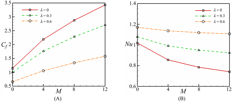
Figure 3.45 Effects of velocity ratio parameter and magnetic parameter on the (A) skin friction coefficient and (B) Nusselt number when Pr = 6.2, ɸ = 0.04, λ = 0.2, Rd = 5, and n = 1.

Figure 3.46 Effect of radiation parameter on the (A) temperature profile and (B) Nusselt number when Pr = 6.2, ɸ = 0.04, and n = 1.
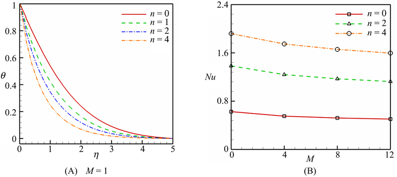
Figure 3.47 Effect of temperature index parameter on the (A) temperature profile and (B) Nusselt number when Pr = 6.2, ɸ = 0.04, and Rd = 5.
3.7. Forced convective heat transfer of magnetic nanofluid in a double-sided, lid-driven cavity with a wavy wall
3.7.1. Problem definition
The schematic of the problem and the related boundary conditions, as well as the mesh of the enclosure that is used in the present CVFEM program are shown in Fig. 3.48 [13]. The enclosure has a width/height aspect ratio of two. The two sidewalls with length  are thermally insulated, whereas the lower flat and upper sinusoidal walls are maintained at constant temperatures Tc and Th, respectively. Under all circumstances, the condition Th > Tc is maintained. The shape of the upper sinusoidal wall profile is assumed to mimic the following pattern [14,15]:

Figure 3.48 (A) Geometry and the boundary conditions and (B) the mesh of enclosure considered in this work.
where a is the dimensionless amplitude of the sinusoidal wall.
The contours of the magnetic field strength are shown in Fig. 3.49. In this study, the magnetic source is located at (1.01 cols, 0.5 rows). The upper wall is the driven lid with a velocity of ULid. The governing equations are similar to those in Section 3.3.1.

Figure 3.49 Contours of the (A) magnetic field strength H, (B) magnetic field intensity component in x direction Hx, and (C) magnetic field intensity component in y direction Hy.
3.7.2. Effects of active parameters
Forced convection heat transfer of a ferronanofluid in the presence of a variable magnetic field is studied using CVFEM. A combination of both the ferrohydrodynamic and the magnetohydrodynamic laws are used to obtain the mathematical model. The enclosure is filled with a Fe3O4-water nanofluid. Calculations are made for various values of the Reynolds numbers (Re = 10 and 100), volume fraction of nanoparticles (ɸ = 0 and 4%), Hartmann number (Ha = 0, 5 and 10), and magnetic number (MnF = 0, 2, 4, 6, and 10). In all calculations, the Prandtl number (Pr), temperature number (ɛ1), and the Eckert number (Ec) are set to be 6.8, 0.0, and 10−5, respectively. CVFEM has been used in this problem. In recent decade, several documents have been published by several authors as application of new numerical methods [16–30].
A comparison of the streamlines between the nanofluid case and the pure fluid case is shown in Fig. 3.50. Adding nanoparticles in the base fluid causes the energy transport to increase. Also, the thermal boundary layer thickness increases with an increase in the volume fraction of the nanofluid. The isotherms and streamlines contours for different values of the Reynolds, Hartmann, and the magnetic numbers are shown in Figs. 3.51 and 3.52. In the absence of the magnetic field at Re = 10, three rotating eddies exist in which the middle one rotates in the clockwise direction, while the other two rotate in the counter clockwise direction. Two thermal plumes are predicted to generate over the hot and cold walls. As the Kelvin force increases, the middle eddy stretches to the left side. In turn, the thermal plumes slant to the left side. However, an increase in the Lorentz force in the absence of the Kelvin force causes the middle eddy to disappear. As the Reynolds number increases, the thermal boundary layer thickness decreases. The middle eddy splits into three small vortices, such that the isotherms become more complex at high Reynolds numbers.

Figure 3.50 Comparison of the streamlines between (A) nanofluid (ɸ = 0.04) and (B) pure fluid (ɸ = 0) when Re = 100, MnF = 10, Ha = 10, Ec = 10−5, ɛ1 = 0, and Pr = 6.8.

Figure 3.51 (A) Isotherms and (B) streamlines contours for different values of Hartmann number and magnetic number when Re = 10.

Figure 3.52 (A) Isotherms and (B) streamlines contours for different values of Hartmann number and magnetic number when Re = 100.
Figs. 3.53 and 3.54 depict that the effects of the magnetic number, Hartmann number, and the Reynolds number on the local and average Nusselt numbers. The corresponding polynomial representation of such a model for the Nusselt number is given by the following relation:
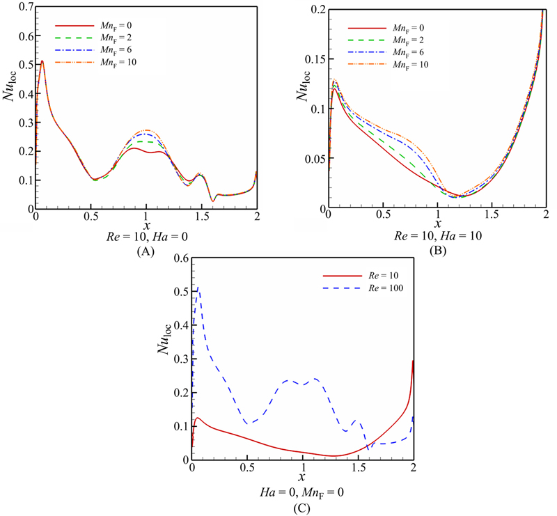
Figure 3.53 Effects of (A–C) Hartmann number, (A–B) Reynolds number, and (C) magnetic number on local Nusselt number (Nuloc) along cold wall.

Figure 3.54 (A–B) Effects of Hartmann number, magnetic number, and Reynolds number on local Nusselt number Nuave along cold wall.
 (3.137)
Table 3.11 shows that values of aij. The thermal boundary layer thickness increases with an increase in the Hartmann number, while it decreases with the augmentation of the magnetic number and the Reynolds number. As a result, the average Nusselt number increases with an increase in the Reynolds number and the magnetic number, while it decreases with an increase in the Hartmann number and the magnetic number. For higher values of the Reynolds number, the effect of the Lorentz force on the Nusselt number becomes more sensible at higher values of the magnetic number. The effects of the magnetic number, Reynolds number, and the Hartmann number on the heat transfer enhancement are shown in Fig. 3.55. The corresponding polynomial representation of such a model for heat transfer enhancement is given by the following relation:
Table 3.11
Constant coefficient for using Eq. (3.137)
| aij | i = 1 | i = 2 | i = 3 | i = 4 | i = 5 | i = 6 |
| j = 1 | 3.090333 | 67.74909 | −0.01146 | 2.709964 | −0.00108 | 0.185167 |
| j = 2 | 0.032216 | 0.292854 | 0.105338 | −0.0021 | −0.00416 | −0.00054 |
| j = 3 | 0.03716 | 0.337792 | −0.01411 | −0.00254 | −0.00108 | 0.00019 |
| j = 4 | −1.89332 | 1.936088 | 0.019527 | −0.10502 | −0.00014 | −0.00391 |
| j = 5 | −4.51078 | 1.390057 | 1.643087 | −0.53284 | −0.5816 | 0.935786 |
| j = 6 | 0.476316 | −0.26171 | 0.953122 | 0.025757 | −0.01112 | 0.028052 |

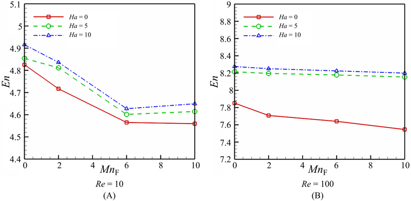
Figure 3.55 (A–B) Effects of Hartmann number, magnetic number, and Reynolds number on heat transfer enhancement.
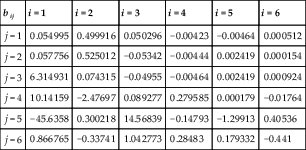
 (3.138)
The values of bij are given in Table 3.12. The heat transfer enhancement decreases with an increase in the magnetic number. The effect of nanoparticles is more pronounced at high Hartmann and Reynolds numbers. This observation can be explained by noting that at high values of these parameters, the heat transfer is dominant by conduction. Therefore, the addition of high thermal conductivity nanoparticles increases the conduction heat transfer and makes the heat transfer enhancement more effective.
Table 3.12
Constant coefficient for using Eq. (3.138)
| bij | i = 1 | i = 2 | i = 3 | i = 4 | i = 5 | i = 6 |
| j = 1 | 0.054995 | 0.499916 | 0.050296 | −0.00423 | −0.00464 | 0.000512 |
| j = 2 | 0.057756 | 0.525012 | −0.05342 | −0.00444 | 0.002419 | 0.000154 |
| j = 3 | 6.314931 | 0.074315 | −0.04955 | −0.00464 | 0.002419 | 0.000924 |
| j = 4 | 10.14159 | −2.47697 | 0.089277 | 0.279585 | 0.000179 | −0.01764 |
| j = 5 | −45.6358 | 0.300218 | 14.56839 | −0.14793 | −1.29913 | 0.40536 |
| j = 6 | 0.866765 | −0.33741 | 1.042773 | 0.28483 | 0.179332 | −0.441 |
..................Content has been hidden....................
You can't read the all page of ebook, please click here login for view all page.