6.6. Magnetohydrodynamic free convection of Al2O3–water nanofluid considering thermophoresis and Brownian motion effects–water nanofluid considering thermophoresis and Brownian motion effects

Search in book...
Toggle Font Controls
Create new playlist

Name your new playlist

Playlist description (optional)
Sign In

Email address

Password

Forgot Password?

or

Continue with Facebook

Continue with Google
Sign Up

Full Name

Email address

Confirm Email Address

Password

or

Continue with Facebook

Continue with Google

6.6. Magnetohydrodynamic free convection of Al₂O₃–water nanofluid considering thermophoresis and Brownian motion effects

6.6.1. Problem definition

The schematic diagram and the mesh of the semiannulus enclosure used in the present CVFEM program are shown in Fig. 6.31 [12]. The inner and outer walls are maintained at constant temperatures T_h and T_c, respectively, while the two other walls are thermally insulated. Also, the boundary conditions of concentration are similar to temperature. It is also assumed that the uniform magnetic field (

\vec{B} = B_{x} \vec{e_{x}} + B_{y} \vec{e_{y}}

$\vec{B} = B_{x} \vec{e_{x}} + B_{y} \vec{e_{y}}$

) of constant magnitude

B = \sqrt{B_{x}^{2} + B_{y}^{2}}

$B = \sqrt{B_{x}^{2} + B_{y}^{2}}$

is applied, where

\vec{e_{x}}

$\vec{e_{x}}$

and

\vec{e_{y}}

$\vec{e_{y}}$

are unit vectors in the Cartesian coordinate system. The orientation of the magnetic field forms an angle λ with horizontal axis such that λ = B_x/B_y. The electric current J and the electromagnetic force F are defined by

J = σ (\vec{V} \times \vec{B})

$J = σ (\vec{V} \times \vec{B})$

and

F = σ (\vec{V} \times \vec{B}) \times \vec{B}

$F = σ (\vec{V} \times \vec{B}) \times \vec{B}$

, respectively.

Table 6.3

Constant coefficient for using Eq. (6.70)

a_ij	i = 1	i = 2	i = 3	i = 4	i = 5	i = 6
j = 1	4.080931	−0.10849	10.44936	−0.10891	0.417974	−0.03188
j = 2	7.809771	−2.67057	2.414376	0.452514	0.790997	−0.97843
j = 3	8.465516	0.484181	−4.13987	−0.01217	0.4827	0.145098

Table 6.4

Constant coefficient for using Eq. (6.80)

b_ij	i = 1	i = 2	i = 3	i = 4	i = 5	i = 6
j = 1	9.333563	−0.00506	4.537482	0.195157	−2.33844	0.508573
j = 2	3.204931	5.085197	0.530967	−0.77932	0.195157	−0.07679
j = 3	−134.848	14.51322	11.03078	−0.10825	0.060356	−1.0671

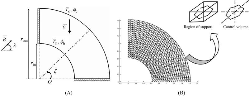
Figure 6.31 (A) Geometry and the boundary conditions; (B) the mesh of enclosure considered in this work.

The nanofluid’s density, ρ, is

$\begin{array}{l} ρ = φ ρ_{p} + (1 - φ) ρ_{f} \\ ≅ φ ρ_{p} + (1 - φ) \{ρ_{f_{0}} (1 - β (T - T_{c})\} \end{array}$ $\begin{array}{l} ρ = φ ρ_{p} + (1 - φ) ρ_{f} \\ ≅ φ ρ_{p} + (1 - φ) \{ρ_{f_{0}} (1 - β (T - T_{c})\} \end{array}$

(6.81)

where ρ_f is the base fluid’s density, T_c is a reference temperature,

ρ_{f_{0}}

$ρ_{f_{0}}$

is the base fluid’s density at the reference temperature, and β is the volumetric coefficient of expansion. Taking the density of base fluid as that of the nanofluid, as adopted by [13], the density ρ in Eq. (6.81), thus, becomes

$ρ ≅ φ ρ_{p} + (1 - φ) \{ρ_{0} (1 - β (T - T_{c})\}$ $ρ ≅ φ ρ_{p} + (1 - φ) \{ρ_{0} (1 - β (T - T_{c})\}$

(6.82)

where ρ₀ is the nanofluid’s density at the reference temperature.

The continuity, momentum under Boussinesq approximation, and energy equations for the laminar and steady-state natural convection in a two-dimensional enclosure can be defined in dimensional form as follows:

$\frac{\partial u}{\partial x} + \frac{\partial v}{\partial y} = 0$ $\frac{\partial u}{\partial x} + \frac{\partial v}{\partial y} = 0$

(6.83)

$ρ_{f} \{u \frac{\partial u}{\partial x} + v \frac{\partial u}{\partial y}\} = - \frac{\partial P}{\partial x} + μ (\frac{\partial^{2} u}{\partial x^{2}} + \frac{\partial^{2} u}{\partial y^{2}}) + σ B^{2} (v \sin λ \cos λ - u \sin^{2} λ)$ $ρ_{f} \{u \frac{\partial u}{\partial x} + v \frac{\partial u}{\partial y}\} = - \frac{\partial P}{\partial x} + μ (\frac{\partial^{2} u}{\partial x^{2}} + \frac{\partial^{2} u}{\partial y^{2}}) + σ B^{2} (v \sin λ \cos λ - u \sin^{2} λ)$

(6.84)

$\begin{array}{l} ρ_{f} \{u \frac{\partial v}{\partial x} + v \frac{\partial v}{\partial y}\} = - \frac{\partial P}{\partial y} + μ (\frac{\partial^{2} v}{\partial x^{2}} + \frac{\partial^{2} v}{\partial y^{2}}) - (φ - φ_{c}) (ρ_{p} - ρ_{f_{0}}) g \\ + (1 - φ_{c}) ρ_{f_{0}} (T - T_{c}) g + σ B^{2} (u \sin λ \cos λ - v \cos^{2} λ) \end{array}$ $\begin{array}{l} ρ_{f} \{u \frac{\partial v}{\partial x} + v \frac{\partial v}{\partial y}\} = - \frac{\partial P}{\partial y} + μ (\frac{\partial^{2} v}{\partial x^{2}} + \frac{\partial^{2} v}{\partial y^{2}}) - (φ - φ_{c}) (ρ_{p} - ρ_{f_{0}}) g \\ + (1 - φ_{c}) ρ_{f_{0}} (T - T_{c}) g + σ B^{2} (u \sin λ \cos λ - v \cos^{2} λ) \end{array}$

(6.85)

$u \frac{\partial T}{\partial x} + v \frac{\partial T}{\partial y} = α (\frac{\partial^{2} T}{\partial x^{2}} + \frac{\partial^{2} T}{\partial y^{2}}) + \frac{{(ρ c)}_{p}}{{(ρ c)}_{f}} [\begin{array}{l} D_{B} \{\frac{\partial φ}{\partial x} . \frac{\partial T}{\partial x} + \frac{\partial φ}{\partial y} . \frac{\partial T}{\partial y}\} \\ + (D_{T} / T_{c}) \{{(\frac{\partial T}{\partial x})}^{2} + {(\frac{\partial T}{\partial y})}^{2}\} \end{array}]$ $u \frac{\partial T}{\partial x} + v \frac{\partial T}{\partial y} = α (\frac{\partial^{2} T}{\partial x^{2}} + \frac{\partial^{2} T}{\partial y^{2}}) + \frac{{(ρ c)}_{p}}{{(ρ c)}_{f}} [\begin{array}{l} D_{B} \{\frac{\partial φ}{\partial x} . \frac{\partial T}{\partial x} + \frac{\partial φ}{\partial y} . \frac{\partial T}{\partial y}\} \\ + (D_{T} / T_{c}) \{{(\frac{\partial T}{\partial x})}^{2} + {(\frac{\partial T}{\partial y})}^{2}\} \end{array}]$

(6.86)

$u \frac{\partial φ}{\partial x} + v \frac{\partial φ}{\partial y} = D_{B} \{\frac{\partial^{2} φ}{\partial x^{2}} + \frac{\partial^{2} φ}{\partial y^{2}}\} + (\frac{D_{T}}{T_{c}}) \{\frac{\partial^{2} T}{\partial x^{2}} + \frac{\partial^{2} T}{\partial y^{2}}\}$ $u \frac{\partial φ}{\partial x} + v \frac{\partial φ}{\partial y} = D_{B} \{\frac{\partial^{2} φ}{\partial x^{2}} + \frac{\partial^{2} φ}{\partial y^{2}}\} + (\frac{D_{T}}{T_{c}}) \{\frac{\partial^{2} T}{\partial x^{2}} + \frac{\partial^{2} T}{\partial y^{2}}\}$

(6.87)

Boundary conditions are as follows:

$\begin{array}{l} T = T_{h}, φ = φ_{h} on the inner circular boundary \\ T = T_{c}, φ = φ_{c} on the outer circular boundary \\ \partial T / \partial n = \partial φ / \partial n = 0.0 on two other insulation boundaries \\ ψ = 0 all the solid boundaries \end{array}$ $\begin{array}{l} T = T_{h}, φ = φ_{h} on the inner circular boundary \\ T = T_{c}, φ = φ_{c} on the outer circular boundary \\ \partial T / \partial n = \partial φ / \partial n = 0.0 on two other insulation boundaries \\ ψ = 0 all the solid boundaries \end{array}$

(6.88)

The stream function and vorticity are defined as follows:

$u = \frac{\partial ψ}{\partial y}, v = - \frac{\partial ψ}{\partial x}, ω = \frac{\partial v}{\partial x} - \frac{\partial u}{\partial y}$ $u = \frac{\partial ψ}{\partial y}, v = - \frac{\partial ψ}{\partial x}, ω = \frac{\partial v}{\partial x} - \frac{\partial u}{\partial y}$

(6.89)

The stream function satisfies the continuity Eq. (6.83). The vorticity equation is obtained by eliminating the pressure between the two momentum equations, that is, by taking y-derivative of Eq. (6.84) and subtracting from it the x-derivative of Eq. (6.85). Also, the following nondimensional variables should be introduced:

$X = \frac{x}{L}, Y = \frac{y}{L}, Ω = \frac{ω L^{2}}{α}, Ψ = \frac{ψ}{α}, Θ = \frac{T - T_{c}}{T_{h} - T_{c}}, Φ = \frac{φ - φ_{c}}{φ_{h} - φ_{c}}, U = \frac{u L}{α}, V = \frac{v L}{α}$ $X = \frac{x}{L}, Y = \frac{y}{L}, Ω = \frac{ω L^{2}}{α}, Ψ = \frac{ψ}{α}, Θ = \frac{T - T_{c}}{T_{h} - T_{c}}, Φ = \frac{φ - φ_{c}}{φ_{h} - φ_{c}}, U = \frac{u L}{α}, V = \frac{v L}{α}$

(6.90)

where, in Eq. (6.90), L = r_out−r_in = r_in.

By using these dimensionless parameters, the equations become

$\begin{array}{l} [\frac{\partial Ψ}{\partial Y} \frac{\partial Ω}{\partial X} - \frac{\partial Ψ}{\partial X} \frac{\partial Ω}{\partial Y}] = \Pr (\frac{\partial^{2} Ω}{\partial X^{2}} + \frac{\partial^{2} Ω}{\partial Y^{2}}) + \Pr R a (\frac{\partial Θ}{\partial X} - N r \frac{\partial Φ}{\partial X}) \\ + H a^{2} \Pr (- \frac{δ V}{δ Y} \tan λ + \frac{δ U}{δ Y} \tan^{2} λ + \frac{δ U}{δ X} \tan λ - \frac{δ V}{δ X}) \end{array}$ $\begin{array}{l} [\frac{\partial Ψ}{\partial Y} \frac{\partial Ω}{\partial X} - \frac{\partial Ψ}{\partial X} \frac{\partial Ω}{\partial Y}] = \Pr (\frac{\partial^{2} Ω}{\partial X^{2}} + \frac{\partial^{2} Ω}{\partial Y^{2}}) + \Pr R a (\frac{\partial Θ}{\partial X} - N r \frac{\partial Φ}{\partial X}) \\ + H a^{2} \Pr (- \frac{δ V}{δ Y} \tan λ + \frac{δ U}{δ Y} \tan^{2} λ + \frac{δ U}{δ X} \tan λ - \frac{δ V}{δ X}) \end{array}$

(6.91)

$\frac{\partial Ψ}{\partial Y} \frac{\partial Θ}{\partial X} - \frac{\partial Ψ}{\partial X} \frac{\partial Θ}{\partial Y} = (\frac{\partial^{2} Θ}{\partial X^{2}} + \frac{\partial^{2} Θ}{\partial Y^{2}}) + N b (\frac{\partial Φ}{\partial X} \frac{\partial Θ}{\partial X} + \frac{\partial Φ}{\partial Y} \frac{\partial Θ}{\partial Y}) + N t ({(\frac{\partial Θ}{\partial X})}^{2} + {(\frac{\partial Θ}{\partial Y})}^{2})$ $\frac{\partial Ψ}{\partial Y} \frac{\partial Θ}{\partial X} - \frac{\partial Ψ}{\partial X} \frac{\partial Θ}{\partial Y} = (\frac{\partial^{2} Θ}{\partial X^{2}} + \frac{\partial^{2} Θ}{\partial Y^{2}}) + N b (\frac{\partial Φ}{\partial X} \frac{\partial Θ}{\partial X} + \frac{\partial Φ}{\partial Y} \frac{\partial Θ}{\partial Y}) + N t ({(\frac{\partial Θ}{\partial X})}^{2} + {(\frac{\partial Θ}{\partial Y})}^{2})$

(6.92)

$\frac{\partial Ψ}{\partial Y} \frac{\partial Φ}{\partial X} - \frac{\partial Ψ}{\partial X} \frac{\partial Φ}{\partial Y} = \frac{1}{L e} (\frac{\partial^{2} Φ}{\partial X^{2}} + \frac{\partial^{2} Φ}{\partial Y^{2}}) + \frac{N t}{N b L e} (\frac{\partial^{2} Θ}{\partial X^{2}} + \frac{\partial^{2} Θ}{\partial Y^{2}})$ $\frac{\partial Ψ}{\partial Y} \frac{\partial Φ}{\partial X} - \frac{\partial Ψ}{\partial X} \frac{\partial Φ}{\partial Y} = \frac{1}{L e} (\frac{\partial^{2} Φ}{\partial X^{2}} + \frac{\partial^{2} Φ}{\partial Y^{2}}) + \frac{N t}{N b L e} (\frac{\partial^{2} Θ}{\partial X^{2}} + \frac{\partial^{2} Θ}{\partial Y^{2}})$

(6.93)

$\frac{\partial^{2} Ψ}{\partial X^{2}} + \frac{\partial^{2} Ψ}{\partial Y^{2}} = - Ω$ $\frac{\partial^{2} Ψ}{\partial X^{2}} + \frac{\partial^{2} Ψ}{\partial Y^{2}} = - Ω$

(6.94)

where thermal Rayleigh number, the buoyancy ratio number, Prandtl number, the Brownian motion parameter, the thermophoretic parameter, Lewis number, and Hartmann number of nanofluid are defined as

R a = (1 - φ_{c}) ρ_{f_{0}} g β L^{3} (T_{h} - T_{c}) / (μ α)

$R a = (1 - φ_{c}) ρ_{f_{0}} g β L^{3} (T_{h} - T_{c}) / (μ α)$

N r = (ρ_{p} - ρ_{0}) (φ_{h} - φ_{c}) / [(1 - φ_{c}) ρ_{f_{0}} β L (T_{h} - T_{c})]

$N r = (ρ_{p} - ρ_{0}) (φ_{h} - φ_{c}) / [(1 - φ_{c}) ρ_{f_{0}} β L (T_{h} - T_{c})]$

\Pr = μ / ρ_{f} α, N b = {(ρ c)}_{p} D_{B}

$\Pr = μ / ρ_{f} α, N b = {(ρ c)}_{p} D_{B}$

(φ_{h} - φ_{c}) / ({(ρ c)}_{f} α)

$(φ_{h} - φ_{c}) / ({(ρ c)}_{f} α)$

N t = {(ρ c)}_{p} D_{T} (T_{h} - T_{c}) / [{(ρ c)}_{f} α T_{c}]

$N t = {(ρ c)}_{p} D_{T} (T_{h} - T_{c}) / [{(ρ c)}_{f} α T_{c}]$

L e = α / D_{B}

$L e = α / D_{B}$

, and

H a = L B_{x} \sqrt{σ / μ}

$H a = L B_{x} \sqrt{σ / μ}$

respectively.

The Eq. (6.94) has been obtained using small temperature gradient in a dilute suspension of nanoparticles. The boundary conditions as shown in Fig. 6.31 are as follows:

$\begin{array}{l} Θ = 1.0, Φ = 1.0 on the inner circular boundary \\ Θ = 0.0, Φ = 0.0 on the outer circular boundary \\ \partial Θ / \partial n = \partial Φ / \partial n = 0.0 on two other insulation boundaries \\ Ψ = 0.0 on all solid boundaries \end{array}$ $\begin{array}{l} Θ = 1.0, Φ = 1.0 on the inner circular boundary \\ Θ = 0.0, Φ = 0.0 on the outer circular boundary \\ \partial Θ / \partial n = \partial Φ / \partial n = 0.0 on two other insulation boundaries \\ Ψ = 0.0 on all solid boundaries \end{array}$

(6.95)

The values of vorticity on the boundary of the enclosure can be obtained using the stream function formulation and the known velocity conditions during the iterative solution procedure.

The local Nusselt number on the hot circular wall can be expressed as

$N u_{loc} = - \frac{\partial Θ}{\partial n}$ $N u_{loc} = - \frac{\partial Θ}{\partial n}$

(6.96)

where n is the direction normal to the inner cylinder surface. The average number on the hot circular wall is evaluated as

$N u_{ave} = \frac{1}{0.5 π} \int_{0}^{0.5 π} N u_{loc} (ζ) d ζ$ $N u_{ave} = \frac{1}{0.5 π} \int_{0}^{0.5 π} N u_{loc} (ζ) d ζ$

(6.97)

The heatlines are adequate tools for visualization and analysis of two-dimensional convection heat transfer, through an extension of the heat flux line concept to include the advection terms. Heat function (H) is defined in terms of the energy equation as

$\frac{\partial H}{\partial Y} = U Θ - \frac{\partial Θ}{\partial X}$ $\frac{\partial H}{\partial Y} = U Θ - \frac{\partial Θ}{\partial X}$

(6.98)

$- \frac{\partial H}{\partial X} = V Θ - \frac{\partial Θ}{\partial Y}$ $- \frac{\partial H}{\partial X} = V Θ - \frac{\partial Θ}{\partial Y}$

(6.99)

6.6.2. Effects of active parameters

MHD effect on natural convection heat transfer in an enclosure filled with nanofluid is investigated numerically using CVFEM. Effects of Hartmann number (Ha = 0, 30, 60, and 100), buoyancy ratio number (Nr = 0.1–4), and Lewis number (Le = 2, 4, 6, and 8) on flow and heat transfer characteristics are examined. Brownian motion parameter of nanofluids (Nb = 0.5), thermophoretic parameter of nanofluids (Nt = 0.5), thermal Rayleigh number (Ra = 10⁵), and Prandtl number (Pr = 10) are fixed.

Effects of Hartmann number, Lewis number, and buoyancy ratio number on isotherms, streamlines, isoconcentration, and heatline contours are shown in Figs. 6.32–6.35. When the magnetic field is imposed on the enclosure, the velocity field suppressed owing to the retarding effect of the Lorenz force. So, intensity of convection weakens significantly. The braking effect of the magnetic field is observed from the maximum stream function value. The core of vortex is shift downward vertically as the Hartmann number increases. Also, imposing magnetic field leads to omit the thermal plume over the inner wall. At high Hartmann number, the conduction heat transfer mechanism is more pronounced. For this reason, the isotherms are parallel to each other. Increasing Hartmann number causes the concentration boundary layer thickness near inner wall to increase.

Figure 6.32 Comparison of the isotherms, streamlines, isoconcentration, and heatline contours for different values of thermal Hartmann number when Nr = 0.1, Le = 8, Nt = Nb = 0.5, Ra = 10⁵, and Pr = 10.

Figure 6.33 Comparison of the isotherms, streamlines, isoconcentration, and heatline contours for different values of thermal Hartmann number when Nr = 4, Le = 8, Nt = Nb = 0.5, Ra = 10⁵, and Pr = 10.

Figure 6.34 Comparison of the isotherms, streamlines, isoconcentration and heatline contours for different values of thermal Hartmann number when Nr = 4, Le = 2, Nt = Nb = 0.5, Ra = 10⁵, and Pr = 10.

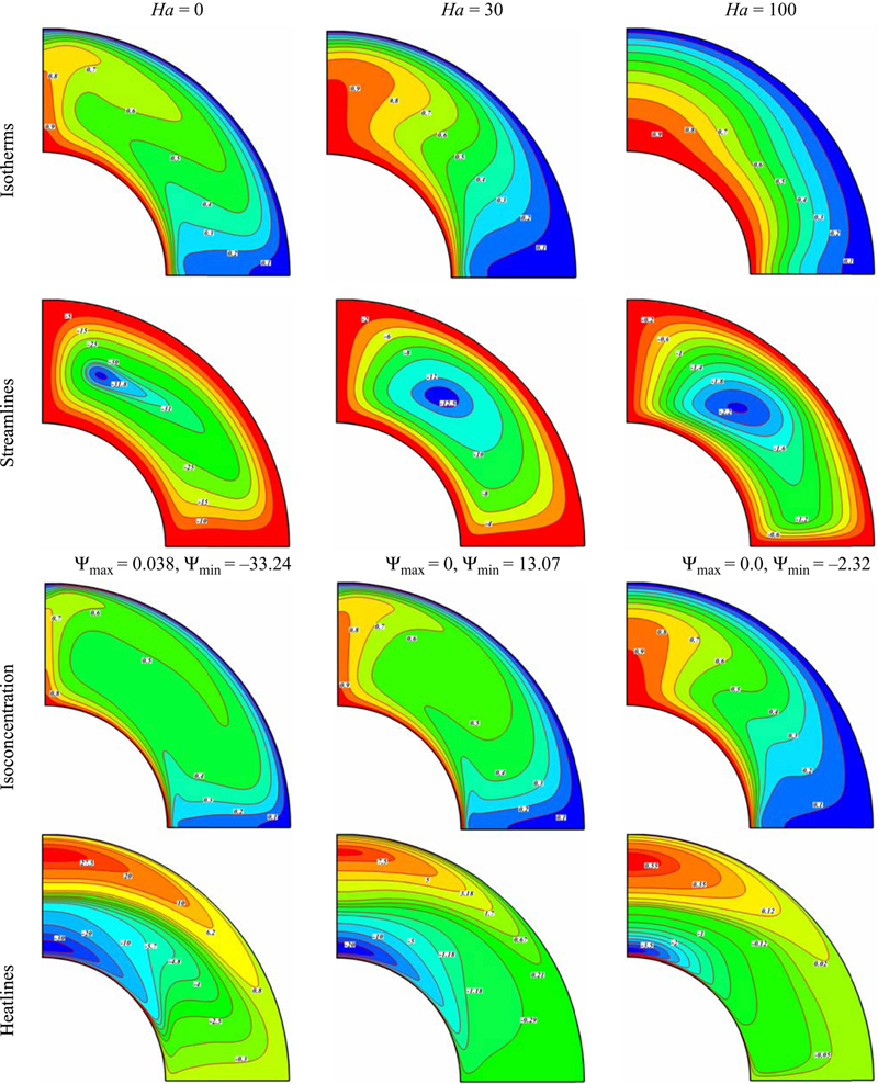
Figure 6.35 Comparison of the isotherms, streamlines, isoconcentration, and heatline contours for different values of thermal Hartmann number when Nr = 0.1, Le = 2, Nt = Nb = 0.5, Ra = 10⁵, and Pr = 10.

The heat flow within the enclosure is displayed using the heat function obtained from conductive heat fluxes (∂Θ/∂X, ∂Θ/∂Y) as well as convective heat fluxes (VΘ, UΘ). Heatlines emanate from hot regimes and end on cold regimes, illustrating the path of heat flow. As seen heatline has two regions rotate in different directions. The lower one is greater than another which means that more heat transfer occurs in this region. As Hartmann number increases, heatlines become weaker because of reduction of heat transfer rate by applying magnetic field. The domination of conduction heat transfer in high Hartmann number can be observed from the heatline patterns as no passive area exists.

It should be mentioned that negative Nr values (opposing buoyancy forces) showed more complex and interesting flow patterns, such as multicells, which is worthy for presentation and discussion. So, in this chapter results for positive Nr (aiding buoyancy forces), where the temperature and species-induced buoyancy forces aid each other, are not considered. For Nr = 0, the species-induced buoyancy force has no effect on flow; the flow is solely driven by the thermal buoyancy force. However, the effect of species-induced buoyancy increases as Nr value increases, and reaches a certain value, where the effect of thermally induced buoyancy becomes negligible in comparison to the solutal one. For small Nr value, the flow is mainly driven by the thermal buoyancy force. When Nr increases, a reverse thermal plume appears at ζ = 90°. This phenomena is due to existing one counter clockwise eddy at this region. By increasing Hartmann number, the two main eddies merged into one counterclockwise eddy. The isconcentrations are more distorted with the increase of solutal forces. As Nr increases, the upper region of heatline counters is divided into two smaller ones, and this new region disappears with the increase of Hartmann number.

The mass flow is given by ψ_max ≈ δ_sv, where the solutal boundary layer thickness is given by δ_s ≈ (Ra Le Nr)^−1/4 and v ≈ (Ra Le Nr)^1/2, so ψ_max ≈ (Ra Le Nr)^1/4. The solutal boundary layer, δ_s, becomes thinner by increasing of Le. Heatlines are found to be more distorted as Le augments.

Effects of Hartmann number, buoyancy ratio number, and Lewis number on local Nusselt number are shown in Fig. 6.36. As seen local Nusselt number increases as buoyancy ratio number increases, but it decreases with the increase of Hartmann number and Lewis number. Generally, as ζ increases local Nusselt number decreases due to increment of thermal boundary layer thickness. In the absence of magnetic field Nu_loc has one local maximum near the bottom wall. The occurrence of maxima for Nu_loc is due to dense heatlines based on conductive heat transport occurring at this portion. This point disappears at high Hartmann number. Local Nusselt number profile has minimum point at ζ = 90° because of existing of thermal plume at this region. Also, this figure shows that effect of Lewis number on Nu_loc is negligible at low buoyancy ratio number.

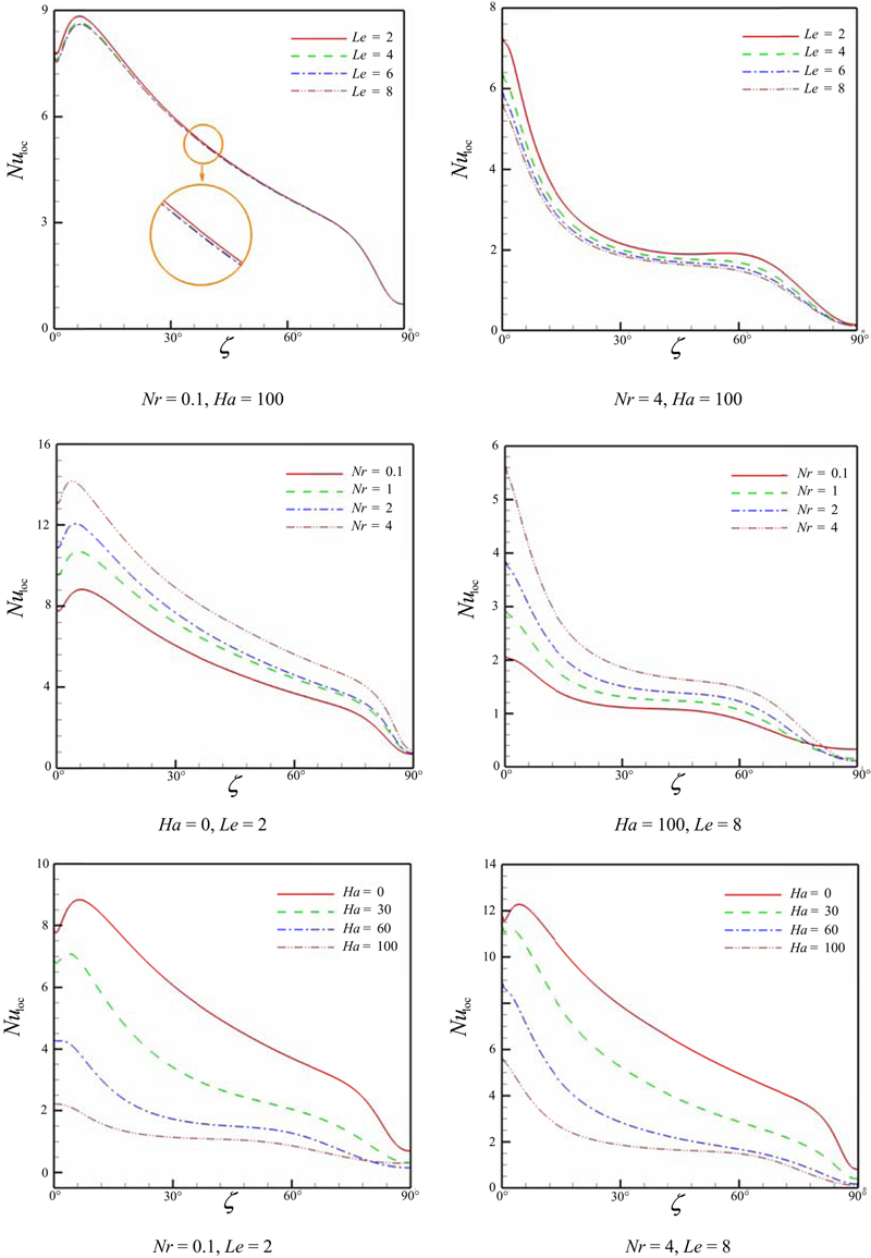
Figure 6.36 Effects of Hartmann number, buoyancy ratio number, and Lewis number on local Nusselt number at Nt = Nb = 0.5, Ra = 10⁵, and Pr = 10.

The corresponding polynomial representation of such model for Nusselt number is as follows:

$\begin{array}{c} N u = a_{13} + a_{23} Y_{1} + a_{33} Y_{2} + a_{43} {Y_{1}}^{2} + a_{53} {Y_{2}}^{2} + a_{63} Y_{1} Y_{2} \\ Y_{1} = a_{11} + a_{21} L e + a_{31} N r + a_{41} L e^{2} + a_{51} N r^{2} + a_{61} L e N r \\ Y_{2} = a_{12} + a_{22} H a^{*} + a_{32} N r + a_{42} H a^{*^{2}} + a_{52} N r^{2} + a_{62} H a^{*} N r \end{array}$ $\begin{array}{c} N u = a_{13} + a_{23} Y_{1} + a_{33} Y_{2} + a_{43} {Y_{1}}^{2} + a_{53} {Y_{2}}^{2} + a_{63} Y_{1} Y_{2} \\ Y_{1} = a_{11} + a_{21} L e + a_{31} N r + a_{41} L e^{2} + a_{51} N r^{2} + a_{61} L e N r \\ Y_{2} = a_{12} + a_{22} H a^{*} + a_{32} N r + a_{42} H a^{*^{2}} + a_{52} N r^{2} + a_{62} H a^{*} N r \end{array}$

(6.100)

where a_ij can be found in Table 6.5, for example, a₂₁ equals to (−0.16499).

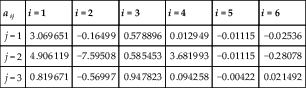
Table 6.5

Constant coefficient for using Eq. (6.100)

a_ij	i = 1	i = 2	i = 3	i = 4	i = 5	i = 6
j = 1	3.069651	−0.16499	0.578896	0.012949	−0.01115	−0.02536
j = 2	4.906119	−7.59508	0.585453	3.681993	−0.01115	−0.28078
j = 3	0.819671	−0.56997	0.947823	0.094258	−0.00422	0.021492

Effects of Hartmann number, buoyancy ratio number, and Lewis number on average Nusselt number are shown in Figs. 6.37 and 6.38. The presence of magnetic field leads the thermal plume to disappear over inner wall and makes the isotherms parallel to each other due to domination of conduction mode of heat transfer. Therefore, average Nusselt number decreases with the increase of Hartmann number. As Lewis number increases, thermal boundary layer thickness increases and in turn Nusselt number decreases. Effect of buoyancy ratio number on Nu_ave is in contrast with Ha and Le. Also, it can be found that effect of Hartmann number and Lewis number is more pronounced at higher values of buoyancy ratio number.

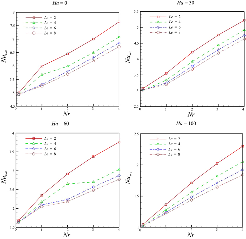
Figure 6.37 Effects of Hartmann number, buoyancy ratio number, and Lewis number on average Nusselt number at Nt = Nb = 0.5, Ra = 10⁵, and Pr = 10.

Figure 6.38 Variation of Nu_ave for various input parameters.

..................Content has been hidden....................

You can't read the all page of ebook, please click here login for view all page.

Table of Contents for 6.6. Magnetohydrodynamic free convection of Al2O3&#8211;water nanofluid considering thermophoresis and Brownian motion effects–water nanofluid considering thermophoresis and Brownian motion effects

Create new playlist

Sign In

Sign Up