
Chapter 6
Nanofluid Flow and Heat Transfer in the Presence of Constant Magnetic Field
Abstract
Natural convection under the influence of a magnetic field has great importance in many industrial applications such as crystal growth, metal casting, and liquid metal cooling blankets for fusion reactors. Existence of magnetic field has a noticeable effect on heat transfer reduction under natural convection, while in many engineering applications increasing heat transfer from solid surfaces is a goal. At this circumstance, the use of nanofluids with higher thermal conductivity can be considered as a promising solution. In this chapter, influence of Lorentz forces on hydrothermal behavior is studied.
Keywords
magnetohydrodynamic
nanofluid
entropy generation
natural convection
CVFEM
LBM
6.1. Entropy generation of nanofluid in the presence of magnetic field using lattice Boltzmann method
6.1.1. Problem definition
The considered physical geometry with related parameters and coordinates are shown in Fig. 6.1A. A rectangular body with height t and width H/2 is placed in the center of the enclosure, and is supposed to be isothermal at higher temperature than two vertical isothermal walls, while the top and bottom walls are insulated. In addition, it is also assumed that the uniform magnetic field ( ) of constant magnitude
  is applied, where
  and
and  are unit vectors in the Cartesian coordinate system. The orientation of the magnetic field forms an angle θM with horizontal axis such that θM = Bx/By. The electric current J and the electromagnetic force F are defined by
  and
and  , respectively. In this section, θM is equal to zero [1].
) of constant magnitude is applied, where 
Figure 6.1 (A) Geometry of the problem; (B) discrete velocity set of two-dimensional nine-velocity (D2Q9) model.
One of the novel computational fluid dynamics (CFD) methods, which is solved Boltzmann equation to simulate the flow instead of solving the Navier–Stokes equations, is called lattice Boltzmann methods (LBM) [or thermal lattice Boltzmann methods (TLBM)]. LBM has several advantages such as simple calculation procedure and efficient implementation for parallel computation, over other conventional CFD methods, because of its particulate nature and local dynamics. The thermal LB model utilizes two distribution functions, f and g, for the flow and temperature fields, respectively. It uses modeling of movement of fluid particles to capture macroscopic fluid quantities such as velocity, pressure, and temperature. In this approach, the fluid domain discretized to uniform Cartesian cells. Each cell holds a fixed number of distribution functions, which represent the number of fluid particles moving in these discrete directions. The D2Q9 model was used, and values of w0 = 4/9 for |c0| = 0 (for the static particle), w1–4 = 1/9 for |c1–4| = 1, and w5–9 = 1/36 for  are assigned in this model (Fig. 6.1B). The density and distribution functions, that is, the f and g, are calculated by solving the lattice Boltzmann equation, which is a special discretization of the kinetic Boltzmann equation. After introducing BGK approximation, the general form of lattice Boltzmann equation with external force is as follows.
For the flow field:
 (6.1)
(6.1)For the temperature field:
 (6.2)
(6.2)where ∆t denotes lattice time step, ci is the discrete lattice velocity in direction i, Fk is the external force in direction of lattice velocity, and τv and τC denote the lattice relaxation time for the flow and temperature fields. The kinetic viscosity υ and the thermal diffusivity α are defined in terms of their respective relaxation times, that is,  and
and  , respectively. Note that the limitation 0.5 < τ should be satisfied for both relaxation times to ensure that viscosity and thermal diffusivity are positive. Furthermore, the local equilibrium distribution function determines the type of problem that needs to be solved. It also models the equilibrium distribution functions, which are calculated with Eqs. (6.3) and (6.4) for flow and temperature fields, respectively.
 (6.3)
(6.3)
 (6.4)
(6.4)where wi is a weighting factor and ρ is the lattice fluid density.
To incorporate buoyancy forces and magnetic forces in the model, the force term in the Eq. (6.2) needs to calculate as follows [1]:
 (6.5)
(6.5)where A is  ,
,  is Hartmann number, and θM is the direction of the magnetic field. For natural convection, the Boussinesq approximation is applied and radiation heat transfer is negligible. To ensure that the code works in near incompressible regime, the characteristic velocity of the flow for natural
  regime must be small compared with the fluid speed of sound. In this chapter, the characteristic velocity selected as 0.1 of sound speed.
, is Hartmann number, and θM is the direction of the magnetic field. For natural convection, the Boussinesq approximation is applied and radiation heat transfer is negligible. To ensure that the code works in near incompressible regime, the characteristic velocity of the flow for natural Finally, macroscopic variables calculate with the following formula:
 (6.6)
(6.6)According to Bejan [2], one can find the volumetric entropy generation rate as
where HTI is the irreversibility due to heat transfer in the direction of finite temperature gradients and FFI is the contribution of fluid friction irreversibility to the total generated entropy.
In terms of the primitive variables, HTI and FFI become
 (6.8)
(6.8)One can also define the Bejan number, Be, as
 (6.9)
(6.9)Note that a Be value more/less than 0.5 shows that the contribution of HTI to the total entropy generation is higher/lower than that of FFI. The limiting value of Be = 1 shows that the only active entropy generation mechanism is HTI, while Be = 0 represents no HTI contribution.
The dimensionless form of entropy generation rate, Ns, is defined as
 (6.10)
where one finds that
 (6.11)
where the dimensionless temperature difference is defined as
 (6.12)
The dimensionless viscous dissipation function, addressed in Eq. (6.11), takes the following form:
 (6.13)
Here, Ge is the Gebhart number which is defined as [3]
 (6.14)
Average Ns is denoted by <Ns>, where the angle brackets show an average taken over the area, as
 (6.15)
Selecting the fluid, trapped between the heated plate and the cavity, as the thermodynamic system, one observes that the amount of heat entered through the heated plate is equal to the one transferred to the surroundings via the isothermal walls. Moreover, one notes that the total volumetric entropy generation rate is obtainable as
 (6.16)
where, in terms of Nu, it reads
 (6.17)
Applying perturbation techniques for small values of Ω, say Ω<<1, one has
 (6.18)
The dimensionless entropy generation number can be obtained as
 (6.19)
To simulate the nanofluid by the LBM, because of the interparticle potentials and other forces on the nanoparticles, the nanofluid behaves differently from the pure liquid from the mesoscopic point of view and is of higher efficiency in energy transport as well as better stabilization than the common solid–liquid mixture. For modeling the nanofluid because of changing in the fluid thermal conductivity, density, heat capacitance, and thermal expansion, some of the governed equations should change. The effective density (ρnf), the effective heat capacity (ρCp)nf, thermal expansion (ρβ)nf, and electrical conductivity (σ)nf of the nanofluid are defined as
 (6.23)
where φ is the solid volume fraction of the nanoparticles and subscripts f, nf, and s stand for base fluid, nanofluid, and solid, respectively.
 (6.24)
 (6.25)
To compare total heat transfer rate, Nusselt number is used. The average Nusselt numbers are defined as follows:
 (6.26)
6.1.2. Effects of active parameters
In this chapter, LBM is used to investigate the natural convection in a square enclosure filled with CuO–water nanofluid in the presence of magnetic field. A body is placed at the center of enclosure. Calculations are made for various values of Hartmann number (Ha = 0–100), volume fraction of nanoparticle (φ = 0–0.04), and Rayleigh number (Ra = 103, 104, and 105) when height of rectangular body (L/t = 10) and Prandtl number (Pr = 6.8).
The effects of nanoparticles on streamlines and isotherms are shown in Fig. 6.2. By adding nanoparticle, the absolute values of stream functions indicate that the strength of flow decreases. Although thermal boundary layer thickness decreases with adding nanoparticle in the base fluid, Nusselt number increases with the increase of nanofluid volume fraction because of increment in thermal conductivity. Fig. 6.3 shows the isotherms and streamlines for different Rayleigh numbers. In general, the heated lighter fluid is lifted and moves upward along the hot surface of the body and the vertical symmetry line until it encounters the cold top wall. Then the fluid becomes gradually colder and denser while it moves horizontally outward in contact with the cold top wall. Consequently, the cooled denser fluid descends along the cold side walls. For Ra = 103, the heat transfer in the enclosure is mainly dominated by the conduction mode. The circulation of the flow shows two overall rotating symmetric eddies with two inner vortices, respectively, as shown in Fig. 6.3 for the streamlines. At Ra = 104, the patterns of the isotherms and streamlines are about the same as those for Ra = 103. However, a careful observation indicates that the thermal boundary layer on the bottom part of the body is thinner than that on the opposite side, and the inner lower vortex slightly becomes smaller in size and weaker in strength compared with the upper one because the effect of convection on heat transfer and flow increases with the increase of the Rayleigh number. As the Rayleigh number increases up to 105, the role of convection in heat transfer becomes more significant and consequently the thermal boundary layer on the surface of the body becomes thinner. Also, a plume starts to appear on the top of the body and as a result the isotherms move upward, giving rise to a stronger thermal gradient in the upper part of the enclosure and a much lower thermal gradient in the lower part. In consequence, the dominant flow is in the upper half of the enclosure, and correspondingly the core of the recirculating eddies is located only in the upper half. At this Rayleigh number, the flow filed undergoes a bifurcation where two inner vorticies merge. The flow at the bottom of the enclosure is very weak compared with that at the middle and top regions, which suggests stratification effects in the lower regions of the enclosure.
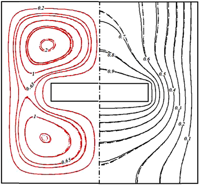
Figure 6.2 Streamlines (left) and isotherms (right) contours between CuO–water nanofluid (φ = 0.04) (−··−) and pure fluid (φ = 0) (––) when Ra = 104, L/t = 10, and Ha = 0.

Figure 6.3 Effects of Rayleigh numbers on streamlines (red) and isotherms (black) contours when L/t = 10, Ha = 0, and φ = 0.04.
Effects of Hartmann number on the streamlines and isotherms are shown in Fig. 6.4. Hartmann number is the ratio of electromagnetic force to the viscous force. Variation of Hartmann number leads to the variation of the Lorentz force due to magnetic field, and the Lorentz force produces more resistance to transport phenomena. Increase of the Hartmann number causes the flow strength decreasing considerably. As the Hartmann number increases, the primary eddy divides into two secondary eddies which are rotate in same direction. Pattern of the isotherms is affected strongly by changing intensity of magnetic field. There is high temperature gradient at the bottom of the body in the absent of magnetic field. With increasing Hartmann number, thermal boundary layer thickness increases at the bottom of the body. The convection is suppressed at the higher Hartmann number. It causes that the plume on the top of the body wall disappears, and isothermal lines become concentric and parallel between the body and the enclosure. It is shown that convection heat transfer becomes weaker and causes the heat transfer mostly dominated by conduction between the cylinders.
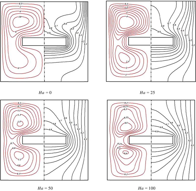
Figure 6.4 Effect of Hartmann number on the streamlines (red) and isotherms (black) when L/t = 10, Ra = 105, and φ = 0.04.
As shown in Table 6.1, at Ra = 103, for all values of Hartmann number, the absolute values of stream function decrease with the increase of nanoparticle volume fraction, whereas for higher value of Rayleigh number, that is, Ra = 104 and Ra = 105, the effect of nanoparticle volume fraction on absolute values of stream function is depended on the value of Hartmann number. In these Rayleigh numbers, when Ha ≤ 50 absolute values of stream function decrease with the decrease of nanoparticle volume fraction, but opposite trend is observed when Ha > 50.
Table 6.1
Effects of the nanoparticle volume fraction and Hartmann number on |ψmax| when L/t = 10
| Ra | ||||
| Ha | φ | 103 | 104 | 105 |
| 0 | 0 | 0.188952 | 2.05299 | 11.48 |
| 0 | 0.04 | 0.18672 | 2.0787 | 11.4451 |
| 50 | 0 | 0.018267 | 0.142036 | 1.57514 |
| 50 | 0.04 | 0.016833 | 0.145037 | 1.55233 |
| 100 | 0 | 0.016523 | 0.046635 | 0.444481 |
| 100 | 0.04 | 0.01025 | 0.044569 | 0.446956 |
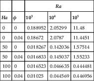
Fig. 6.5 shows the effects of the nanoparticle volume fraction, Rayleigh number, and Hartmann number for Cu–water nanofluids on average Nusselt number ratio  . It can be found that the effect of nanoparticles is more pronounced at low Rayleigh numbers than at high Rayleigh numbers because of greater values of average Nusselt number ratios. This observation can be explained by noting that at low Rayleigh numbers the heat transfer is dominant by conduction. Therefore, the addition of high thermal conductivity nanoparticles will increase the conduction and therefore make the enhancement more effective. When Ha < 75 minimum values of average Nusselt number ratio are obtained for Ra = 105 but when Ha > 75 minimum values of this ratio occurs for Ra = 104.

Figure 6.5 Effects of the active parameters on average Nusselt number ratio when L/t = 10.
Effects of Hartmann number, the nanoparticle volume fraction, Rayleigh number, and dimensionless temperature difference for CuO–water on dimensionless entropy generation number are shown in Fig. 6.6. The dimensionless entropy generation number increases with the increase of nanoparticle volume fraction and Rayleigh number. As shown in Fig. 6.6, <Ns> decreases with the increase of Ω. This fact is in line with the predictions of our Eq. (6.11). This also makes physical sense because, as Ω = Th/Tc − 1, higher values of Ω imply a greater temperature difference (leading to higher heat transfer rates) and consequently boosted HTI values. So decrease in <Ns>, according to  , leads to increase in the total entropy generation. Also, these figures indicate that increasing Hartmann number leads to decrease in dimensionless entropy generation number.

Figure 6.6 Effects of the nanoparticle volume fraction, Hartmann number, Rayleigh number, and dimensionless temperature difference for CuO–water on dimensionless entropy generation number (Ns) (A) when Ra = 105, Ω = 0.06; (B) φ = 0.04, Ω = 0.06; (C) φ = 0.04, Ra = 105 and L/t = 10.
6.2. MHD natural convection in a nanofluid-filled inclined enclosure with sinusoidal wall using CVFEM
6.2.1. Problem definition
Schematic of the problem and the related boundary conditions, as well as the mesh of enclosure which is used in the present control volume-based finite element method (CVFEM) program, are shown in Fig. 6.7 [5]. The enclosure has a width/height aspect ratio of two. The two sidewalls with length H are thermally insulated, whereas the lower flat and upper sinusoidal walls are maintained at constant temperatures Th and Tc, respectively. Under all circumstances Th > Tc condition is maintained. The shape of the upper sinusoidal wall profile is assumed to mimic the following pattern:

Figure 6.7 (A) Geometry and the boundary conditions, and (B) the mesh of enclosure considered in this work.
where a is the dimensionless amplitude of the sinusoidal wall. It is also assumed that the uniform magnetic field () of constant magnitude is applied, where and are unit vectors in the Cartesian coordinate system. The orientation of the magnetic field forms an angle γ with horizontal axis such that γ = Bx/By. The electric current J and the electromagnetic force F are defined by and , respectively.
) of constant magnitude is applied, where The flow is two-dimensional, laminar and incompressible. The radiation, viscous dissipation, induced electric current, and Joule heating are neglected. The magnetic Reynolds number is assumed to be small, so that the induced magnetic field can be neglected compared with the applied magnetic field. The flow is considered to be steady, two-dimensional and laminar. Neglecting displacement currents, induced magnetic field, and using the Boussinesq approximation, the governing equations of heat transfer and fluid flow for nanofluid can be obtained as follows [6]:
 (6.28)
 (6.29)
 (6.30)
 (6.31)
where the effective density (ρnf) and heat capacitance (ρCp)nf of the nanofluid are defined as
where φ is the solid volume fraction of nanoparticles. Thermal diffusivity of the nanofluids is
 (6.34)
and the thermal expansion coefficient of the nanofluids can be determined as
The dynamic viscosity of the nanofluids given is
 (6.36)
The effective thermal conductivity of the nanofluid can be approximated as
 (6.37)
and the effective electrical conductivity of nanofluid was presented as
 (6.38)
The stream function and vorticity are defined as
 (6.39)
The stream function satisfies the continuity Eq. (6.28). The vorticity equation is obtained by eliminating the pressure between the two momentum equations, that is, by taking y-derivative of Eq. (6.29) and subtracting from it the x-derivative of Eq. (6.30). This gives:
 (6.40)
 (6.41)
 (6.42)
By introducing the following nondimensional variables:
 (6.43)
 (6.44)
 (6.45)
 (6.46)
where Raf = gβfL3(Th − Tc)/(αfυf) is the Rayleigh number for the base fluid,  is the Hartmann number, and Prf = υf/αf is the Prandtl number for the base fluid. The boundary conditions as shown in Fig. 6.7 are as follows:
 (6.47)
The values of vorticity on the boundary of the enclosure can be obtained using the stream function formulation and the known velocity conditions during the iterative solution procedure.
The local Nusselt number of the nanofluid along the hot wall can be expressed as
 (6.48)
where n is normal to surface. The average Nusselt number on the hot wall is evaluated as
 (6.49)
6.2.2. Effects of active parameters
Numerical simulations of natural convection nanofluid flow in an enclosure with one sinusoidal wall in the presence of magnetic field were performed using CVFEM. Calculations are made for various values of Hartmann number (Ha = 0, 20, 60, and 100), Rayleigh number (Ra = 103, 104, and 105), volume fraction of nanoparticles (φ = 0, 2, 4, and 6%) and inclination angle (γ = 0, 30, 60, and 90°) at constant dimensionless amplitude of the sinusoidal wall (a = 0.3), and Prandtl number (Pr = 6.2).
Figs. 6.8 and 6.9 show isotherms (up) and streamlines (down) contours for different values of Rayleigh number, Hartmann number, and inclination angle. The figures show that the absolute value of stream function increases with the increase of Rayleigh number, and it decreases as Hartmann number increases. Also, it can be seen that maximum values of |Ψmax| are observed at γ = 90° for Ra = 103 and104, while it is obtained at γ = 60° for Ra = 105. At Ra = 103, for all inclination angles, the isotherms are nearly smooth curves and nearly parallel to each other which follow the geometry of the sinusoidal surfaces; this pattern is the characteristic of conduction dominant mechanism of heat transfer at low Rayleigh numbers. At γ = 0° two counter rotating vortices cores are observed. This bicellular flow pattern divides the cavity into two symmetric parts with respect to vertical center line of the enclosure. By increasing inclination angle, at first the upper vortex becomes stronger, and then at γ = 90°, streamlines become symmetric with respect to horizontal center line of the enclosure. In general, as Rayleigh number increases, the buoyancy-driven circulations inside the enclosure become stronger as it is clear from greater magnitudes of stream function and more distortion appears in the isotherms. When the magnetic field is imposed on the enclosure, the velocity field suppressed owing to the retarding effect of the Lorenz force. So intensity of convection weakens significantly. The braking effect of the magnetic field is observed from the maximum stream function value. Increase of Hartmann number merges two vortexes into one except for γ = 0°. Also, magnetic field disappears the thermal plume over the hot wall and makes the isotherms parallel to each other due to domination of conduction mode of heat transfer.

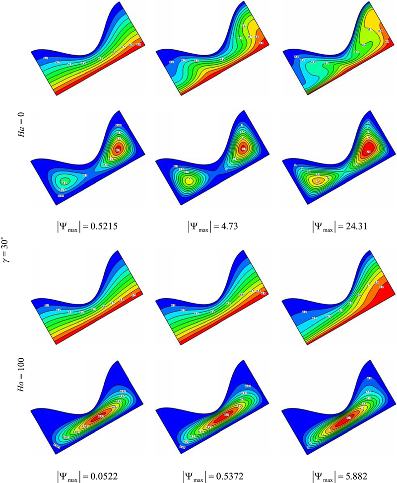
Figure 6.8 Isotherms (up) and streamlines (down) contours for different values of Rayleigh number, Hartmann number and inclination angle at a = 0.3,φ = 0.06, and Pr = 6.2.
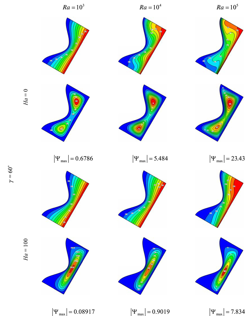

Figure 6.9 Isotherms (up) and streamlines (down) contours for different values of Rayleigh number, inclination angle, and inclination angle at a = 0.3,φ = 0.06, and Pr = 6.2.
Fig. 6.10 depicts the effects of the nanoparticle volume fraction, Hartmann number, inclination angle, and Rayleigh number on local Nusselt number. Generally, increasing the nanoparticles volume fraction and Rayleigh number leads to an increase in local Nusselt number. In the absence of magnetic field, at γ = 0° the local Nusselt profile is symmetric with respect to the vertical center line of the enclosure. But in the presence of magnetic field, because of domination of conduction mechanism, maximum value of local Nusselt number occurs at vertical center line. At γ = 90° the local Nusselt decreases with the increase of S and increasing Hartmann number leads to decrease in Nusselt number. When Ha = 0, the number of extermum in in the local Nusselt number profile is corresponding to the existence of thermal plume.

Figure 6.10 Effects of the nanoparticle volume fraction, Hartmann number, inclination angle, and Rayleigh number on local Nusselt number when (A), (B) Ra = 105, γ = 90°; (C), (D) Ra = 105, φ = 0.06; (E), (F) Ra = 105, φ = 0.06; (G), (H) φ = 0.06, γ = 90°.
Effects of the Hartmann number, Rayleigh number, and inclination angle on the average Nusselt number are shown in Fig. 6.11A–B. Generally, the average Nusselt number increases with the increase of Rayleigh number, while it decreases as Hartmann number increases. At Ra = 105, in the absence of magnetic field, maximum value of average Nusselt number is obtained at γ = 0°, but for higher values of Hartmann number maximum value of Nuave occurs at γ = 90°.

Figure 6.11 Effects of the Hartmann number, Rayleigh number, and inclination angle on the average Nusselt number when (A) Ra = 105; (B) γ = 90° at a = 0.3 and φ = 0.06; (C) Effects of Hartmann number, Rayleigh number, and inclination angle on the ratio of heat transfer enhancement due to addition of nanoparticles a = 0.3.
To estimate the enhancement of heat transfer between the case of φ = 0.06 and the pure fluid (base fluid) case, the enhancement is defined as
 (6.50)
The effects of Hartmann number, Rayleigh number, and inclination angle on heat transfer enhancement ratio are shown in Fig. 6.11C. At Ra = 103, maximum value of enhancement for low Hartmann number is observed at γ = 0°, but for Ha > 20 maximum values of it occur for γ = 90°. Also, it can be seen that for Ra = 104 and 105 maximum values of E are obtained for γ = 60° and γ = 0°, respectively. It is an interesting observation that at Ra = 105 the enhancement in heat transfer for case of γ = 0° increases with the increase of Hartmann number when Ha < 60, while opposite trend is observed for Ha > 60. For other value of inclination angles, enhancement in heat transfer is an increasing function of Hartmann number.
6.3. Effects of MHD on Cu–water nanofluid flow and heat transfer by means of CVFEM
6.3.1. Problem definition
The schematic diagram and the mesh of the semiannulus enclosure used in the present CVFEM program are shown in Fig. 6.12A [7]. The system consists of a circular enclosure with radius of rout, within which an inclined elliptic cylinder is located and rotates from γ = 0° to 90°. Th and Tc are the constant temperatures of the inner and outer cylinders, respectively (Th > Tc). Setting a as the major axis and b as the minor axis of elliptic cylinder, the eccentricity (ɛ) for the inner cylinder is defined as [8]

Figure 6.12 (A) Geometry and the boundary conditions with (B) the mesh of enclosure considered in this work.
In this chapter, for the inner ellipse, the eccentricity and the major axis are 0.9 and 0.8L, respectively.
Also, it is also assumed that the uniform magnetic field ( ) of constant magnitude is applied, where and are unit vectors in the Cartesian coordinate system. The orientation of the magnetic field forms an angle λ with horizontal axis such that λ = Bx/By. The electric current J and the electromagnetic force F are defined by and , respectively. In this chapter, λ is equal to zero.
) of constant magnitude is applied, where The governing equations are similar to those of exist in Section 6.2.1. The local Nusselt number of the nanofluid along the cold wall can be expressed as
 (6.52)
where r is the radial direction. The average Nusselt number on the cold circular wall is evaluated as
 (6.53)
6.3.2. Effects of active parameters
MHD natural convection heat transfer between a circular enclosure and an elliptic cylinder filled with nanofluid is investigated numerically using the CVFEM. Calculations are carried out for constant eccentricity (ɛ = 0.9), major axis (a = 0.8L), and Prandtl (Pr = 6.2) at different values of Rayleigh number (Ra = 103, 104, 105), Hartmann number (Ha = 0, 20, 60, and 100), and inclined angle of inner cylinder (γ = 0, 30, 60, and 90°) and volume fraction of nanoparticles (φ = 0, 2, 4, and 6%).
Isotherms and streamlines for different values of Ra, γ, and Ha are shown in Figs. 6.13 and 6.14. At Ra = 103 the isotherms are parallel to each other and take the form of inner and outer wall, and the stream function magnitude is relatively small which indicates the domination of conduction heat transfer mechanism. Increasing inclination angle leads to an increase in the absolute value of maximum stream function (|Ψmax|) at this Rayleigh number. At γ = 0° the streamlines and isotherms are symmetric with respect to the vertical center line of the enclosure. Each pair cells have two cells. The top vortex is stronger because at this area the hot surface is located beneath the cold one which helps the flow circulation, whereas the arrangement of the existence of cold wall under the hot cylinder at the bottom of the enclosure resists the flow circulation. As γ = 0° increases these two pair cells merge together and form two single-cell different locations inside the enclosure. At γ = 90° again the streamlines pattern become symmetric with respect to the vertical center line of the enclosure. At Ra = 104 the thermal plumbs start to appear over the hot elliptic cylinder. In addition, the stream function values start to growth which show that the convection heat transfer mechanism becomes comparable with conduction. At γ = 0° increase pattern of streamline is similar to that of Ra = 103, but the size of the vortices at the bottom of the enclosure. In addition, the temperature contours become stratified beneath the hot cylinder. With the increase of γ to 30° a secondary vortex appears at the top of the enclosure and the thermal plumb slant to left because of more available space at this area. As the inclination angle of the inner cylinder increases further, this secondary vortex disappears and the stream lines show two main vortices in the enclosure. Also, it can be found that effect of increasing inclination angle on |Ψmax| becomes less pronounced at γ > 30°. When Rayleigh number increases up to Ra = 105 isotherms are totally distorted at the top of the enclosure, while it is stratified at the bottom of the enclosure which shows the heat transfer mechanism is dominated by convection. In the area above the thermal plumb completely formed which impinging the hot fluid to the cold wall of the enclosure, these results in the thermal boundary layer over the cold wall of the enclosure. As seen the secondary vortex exists at γ = 30 and 60° which can the thermal plumb slant to left. Also, as seen maximum value of |Ψmax| occurs at γ = 60°. It is worthwhile mentioning that the effect of magnetic field is to decrease the value of the velocity magnitude throughout the enclosure because the presence of magnetic field introduces a force called the Lorentz force, which acts against the flow if the magnetic field is applied in the normal direction. This type of resisting force slows down the fluid velocity. Increase of Hartmann number makes the core of vortices move toward the horizontal center line. Also magnetic field causes the thermal plume to disappear and makes the isotherms parallel to each other due to domination of conduction mode of heat transfer.

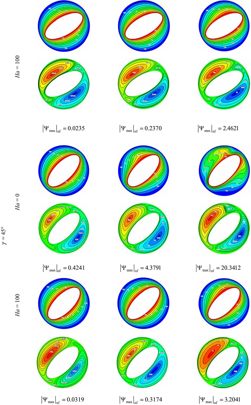
Figure 6.13 Isotherms (up) and streamlines (down) contours for different values of Ra, γ = 0, 30, and 45°, and Ha at φ = 0.06.
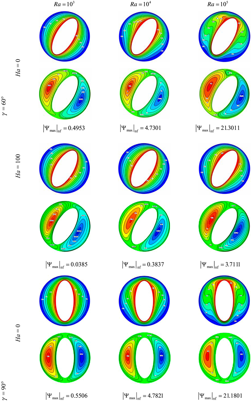
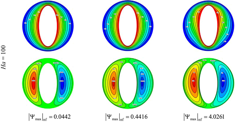
Figure 6.14 Isotherms (up) and streamlines (down) contours for different values of Ra, γ = 60 and 90°, and Ha at φ = 0.06.
Fig. 6.15 shows the distribution of local Nusselt numbers along the surface of the outer circular wall for different inclination angle, Rayleigh number, and Hartmann number. As Rayleigh number increases, the local Nusselt number increases due to increment of convection effect. At Ra = 103 the Nuloc profile is nearly symmetry with respect to the horizontal center line. As Rayleigh number enhances (e.g., Ra = 104 and 105), the Nuloc profile is no longer symmetry and local Nusselt number is considerably small over the bottom wall of the enclosure. Increasing Hartmann number causes local Nusselt number to decreases. These local Nusselt number profiles are more complex due to the presence of thermal plume at the vicinity of the top wall of the enclosure.

Figure 6.15 Effects of the inclination angle, Hartmann number, and Rayleigh number for Cu–water (φ = 0.06) nanofluids on local Nusselt number.
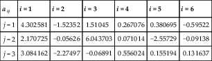
The corresponding polynomial representation of such model for Nusselt number is as follows:
 (6.54)
Table 6.2
Constant coefficient for using Eq. (6.54)
| aij | i = 1 | i = 2 | i = 3 | i = 4 | i = 5 | i = 6 |
| j = 1 | 4.302581 | −1.52352 | 1.51045 | 0.267076 | 0.380695 | −0.59522 |
| j = 2 | 2.170725 | −0.05626 | 6.043703 | 0.071014 | −2.55729 | −0.09138 |
| j = 3 | 3.084162 | −2.27497 | −0.06891 | 0.556024 | 0.155194 | 0.131637 |
Effects of the volume fraction of nanoparticles, inclination angle, Hartmann number, and Rayleigh number on average Nusselt number are shown in Figs. 6.16 and 6.17. Adding nanoparticles leads to an increase in thermal boundary layer thickness; Nusselt number increases because Nusselt number is a multiplication of temperature gradient and the thermal conductivity ratio and reduction in temperature gradient due to the presence of nanoparticles is much smaller than the thermal conductivity ratio. Increasing Rayleigh number is associated with an increase in the heat transfer and the Nusselt number. This is due to stronger convective heat transfer for higher Rayleigh number. Increasing Hartmann number causes Lorenz force to increase and leads to a substantial suppression of the convection. So, Nusselt number has reverse relationship with Hartmann number. Also, these figures show that inclination angle has direct relationship with average Nusselt number. As shown in Fig. 6.16, inclination angle has no significant effect on average Nusselt number at high Hartmann number.

Figure 6.16 Effects of the inclination angle, Hartmann number, and Rayleigh number for Cu–water (φ = 0.06) nanofluids on average Nusselt number.

Figure 6.17 Variation of Nuave for various input parameters.
Heat transfer enhancement ratio due to addition of nanoparticles for different values of Ha, γ, and Ra is shown in Fig. 6.18. Generally, increasing Rayleigh number causes heat transfer enhancement to decrease because of domination of conduction mechanism in low Rayleigh number. Also, Hartmann number is an increasing function of En. As inclination angle increases, En decreases except for Ra = 104. At Ra = 104 maximum values of En occur at γ = 30 and 35° for Ha = 0 and 100, respectively.
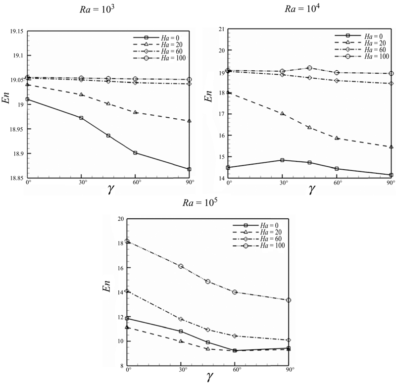
Figure 6.18 Effects of the inclination angle, Hartmann number, and Rayleigh number on the ratio of heat transfer enhancement due to addition of nanoparticles when Pr = 6.2 (Cu–Water case).
6.4. Heat flux boundary condition for nanofluid-filled enclosure in the presence of magnetic field
6.4.1. Problem definition
The physical model along with the important geometrical parameters is shown in Fig. 6.19A. The width and height of the enclosure is L. The outer cylinder is maintained at constant cold temperature Tc, whereas the inner circular wall is under constant heat flux [9]. To assess the shape of inner circular and outer rectangular boundary which consists of the right and top walls, a supper elliptic function can be used as follows:

Figure 6.19 (A) Geometry and the boundary conditions with (B) the mesh of Geometry considered in this work.
 (6.55)
When a = b and  , the geometry becomes a circle. As
  increases from 1, the geometry would approach a rectangle for a # b and square for a = b. It is also assumed that the uniform magnetic field () of constant magnitude is applied, where and are unit vectors in the Cartesian coordinate system. The orientation of the magnetic field forms an angle λ with horizontal axis such that λ = Bx/By. In this chapter, λ equals to zero. The electric current J and the electromagnetic force F are defined by and , respectively.
) of constant magnitude is applied, where The flow is steady, two-dimensional, laminar, and incompressible. The radiation, viscous dissipation, induced electric current, and Joule heating are neglected. The magnetic Reynolds number is assumed to be small, so that the induced magnetic field can be neglected compared with the applied magnetic field. Neglecting displacement currents, induced magnetic field, and using the Boussinesq approximation, the governing equations of heat transfer and fluid flow for nanofluid can be obtained as follows:
 (6.56)
(6.57)
 (6.58)
 (6.59)
where (ρnf), (βnf), (ρCp)nf, and (σnf) are defined as
 (6.60)
(6.61)
 (6.62)
(6.63)The stream function and vorticity are defined as
(6.64)The stream function satisfies the continuity Eq. (6.56). The vorticity equation is obtained by eliminating the pressure between the two momentum equations, that is, by taking y-derivative of Eq. (6.57) and subtracting from it the x-derivative of Eq. (6.58). This gives:
(6.65)
(6.66)
(6.67)By introducing the following nondimensional variables:
 (6.68)
Using the dimensionless parameters, the equations now become:
 (6.69)
 (6.70)
(6.71)where Raf = gβfL4q″/(kf αf vf) is the Rayleigh number for the base fluid,  is the Hartmann number, and Prf = υf /αf is the Prandtl number for the base fluid. The boundary conditions as shown in Fig. 6.19 are as follows:
 (6.72)
The values of vorticity on the boundary of the enclosure can be obtained using the stream function formulation and the known velocity conditions during the iterative solution procedure. The local Nusselt number of the nanofluid along the hot wall can be expressed as
 (6.73)
where r is the radial direction. The average Nusselt number on hot circular wall is evaluated as
 (6.74)
To estimate the enhancement of heat transfer between the case of φ = 0.04 and the pure fluid (base fluid) case, the enhancement is defined as
 (6.75)
The heatlines are adequate tools for visualization and analysis of two-dimensional convection heat transfer, through an extension of the heat flux line concept to include the advection terms. Heat function (H) is defined in terms of the energy equation as
 (6.76)
6.4.2. Effects of active parameters
CVFEM is applied to solve the problem of natural convection in an enclosure filled with Al2O3–water nanofluid in the presence of magnetic field. The effective thermal conductivity and viscosity of nanofluid are calculated by KKL correlation. Calculations are made for various values of volume fraction of nanoparticles (φ = 0%–4%), Rayleigh number (Ra = 103, 104, and 105), aspect ratio (rin/L = 0.2, 0.3, and 0.4), and Hartmann number (Ha = 0–100) at constant Prandtl number (Pr = 6.2).
Comparisons of the isotherms, streamlines, and heatlines for different values of Hartmann number, aspect ratio, and Rayleigh number are shown in Figs. 6.20 and 6.21. By increasing Rayleigh number, the prominent heat transfer mechanism is turned from conduction to convection. Also, it can be seen that increasing aspect ratio leads to decrease in thermal boundary layer thickness and intensity of convection because of domination of conduction heat transfer. When the magnetic field is imposed on the enclosure, the velocity field suppressed owing to the retarding effect of the Lorenz force. So, intensity of convection weakens significantly. The braking effect of the magnetic field is observed from the maximum stream function value. The core vortex is shifted upward vertically as the Hartmann number increases. Also, imposing magnetic field leads to omit the thermal plume over the inner wall. At high Hartmann number, the conduction heat transfer mechanism is more pronounced. For this reason, the isotherms are parallel to each other.

Figure 6.20 Comparison of the isotherms, streamlines, heatlines for different values of Hartmann number and Raleigh number at rin/L = 0.2, φ = 0.04, and Pr = 6.2.

Figure 6.21 Comparison of the isotherms, streamlines, heatlines for different values of Hartmann number and Raleigh number at rin/L = 0.4, φ = 0.04, and Pr = 6.2.
The heat flow within the enclosure is displayed using the heat function obtained from conductive heat fluxes (∂Θ/∂X, ∂Θ/∂Y) as well as convective heat fluxes (VΘ, UΘ). Heatlines emanate from hot regimes and end on cold regimes, illustrating the path of heat flow. The domination of conduction heat transfer in low Rayleigh number and high Hartmann number can be observed from the heatline patterns because no passive area exists. The increase of Ra causes the clustering of heatlines from hot to the cold wall, and generates passive heat transfer area in which heat is rotated without having significant effect on heat transfer between walls.
Distribution of local Nusselt numbers along the surface of the inner circular wall for different aspect ratio, Rayleigh number and Hartmann number are shown in Fig. 6.22. Increasing Rayleigh number and aspect ratio lead to an increase in local Nusselt number, but increasing Hartmann number causes local Nusselt number to decrease.
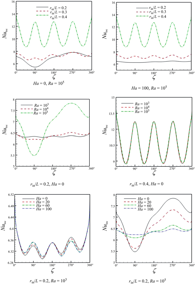
Figure 6.22 Effects of aspect ratio, Rayleigh number, and Hartmann number on local Nusselt number.
Fig. 6.23 shows the effects of aspect ratio, Rayleigh number, and Hartmann number on average Nusselt number. Increasing Hartmann number causes Lorenz force to increase, and leads to a substantial suppression of the convection. So, Nusselt number has reverse relationship with Hartmann number. As aspect ratio increases, space to accelerate the flow inside the cavity decreases. So, thermal boundary layer thickness decreases and in turn 1/θ increases. As volume fraction of nanoparticle increases, thermal diffusivity increases. So, the high values of thermal diffusivity cause the boundary thickness to increase and accordingly decrease 1/θ. Nusselt number is function of 1/θ and knf/kf. Because the reduction in 1/θ due to the presence of nanoparticles is much smaller than thermal conductivity ratio therefore an augment in Nusselt number is taken place by increasing the volume fraction of nanoparticles. The distance between cold and hot walls decreases with the increase of aspect ratio. So, Nusselt number decreases with the increase of rin/L.

Figure 6.23 Effects of aspect ratio, Rayleigh number, and Hartmann number on average Nusselt number.
The heat transfer enhancement ratio due to addition of nanoparticles for different values of rin/L, Ha, and Ra is shown in Fig. 6.24. Heat transfer enhancement ratio has direct relationship with Hartmann number and aspect ratio, but has reverse relationship with Rayleigh number. This observation is due to domination of conduction heat transfer in low Rayleigh number and high Hartmann number or aspect ratio. Therefore, the addition of high thermal conductivity nanoparticles will increase the conduction and make the enhancement more effective.

Figure 6.24 Effects of aspect ratio, Rayleigh number, and Hartmann number on heat transfer enhancement.
6.5. Magnetic field effect on nanofluid flow and heat transfer using KKL model
6.5.1. Problem definition
The physical model along with the important geometrical parameters and the mesh of the enclosure used in the present CVFEM program are shown in Fig. 6.25 [10]. The width and height of the enclosure is H. The right and top wall of the enclosure are maintained at constant cold temperatures Tc, whereas the inner circular hot wall is maintained at constant hot temperature Th and the two bottom and left walls with the length of H/2 are thermally isolated. Under all cases Th > Tc condition is maintained. In this section rin/rout = 0.75. It is also assumed that the uniform magnetic field () of constant magnitude is applied, where and are unit vectors in the Cartesian coordinate system [11]. The governing equations are similar to those of exist in Section 6.4.1. The local Nusselt number of the nanofluid along the hot wall can be expressed as
) of constant magnitude is applied, where 
Figure 6.25 (A) Geometry and the boundary conditions with (B) the mesh of enclosure considered in this work.
 (6.77)
where r is the radial direction. The average Nusselt number on hot circular wall is evaluated as
 (6.78)
6.5.2. Effects of active parameters
In this chapter, MHD effect on natural convection heat transfer in an L-shape inclined enclosure filled with nanofluid is investigated numerically using the CVFEM. The fluid in the enclosure is Al2O3–water nanofluid. Calculations are made for various values of Hartmann number (Ha = 0, 20, 60, and 100), volume fraction of nanoparticle (φ = 0 and 4%), Rayleigh number (Ra = 103, 104, and 105), inclination angle (γ = −90, −60, −30, and 0°), and constant Prandtl number (Pr = 6.2).
Comparisons of the isotherms, streamlines, and heatlines for different values of Hartmann number, inclined angles, and Rayleigh number are shown in Figs. 6.26 and 6.27. At Ra = 103, the isotherms are parallel to each other and take the shape of enclosure which is the main characteristic of conduction heat transfer mechanism. As Rayleigh number increases, the isotherms become more distorted and the stream function values enhance which is due to the domination of convective heat transfer mechanism at higher Rayleigh numbers. At Ra = 105, thermal plume appears on the hot circular wall and three vortices exist in streamline. By increasing |ζ|, these vortices merge into one eddy. As |ζ| increases, the hot wall locates on the cold wall. So, convective heat transfer becomes weak and in turn Nusselt number decreases with the increase of |ζ|.


Figure 6.26 Comparison of the isotherms, streamlines, and heatlines for different values of Hartmann number and inclination angle at Ra = 103, φ = 0.04, and Pr = 6.2.

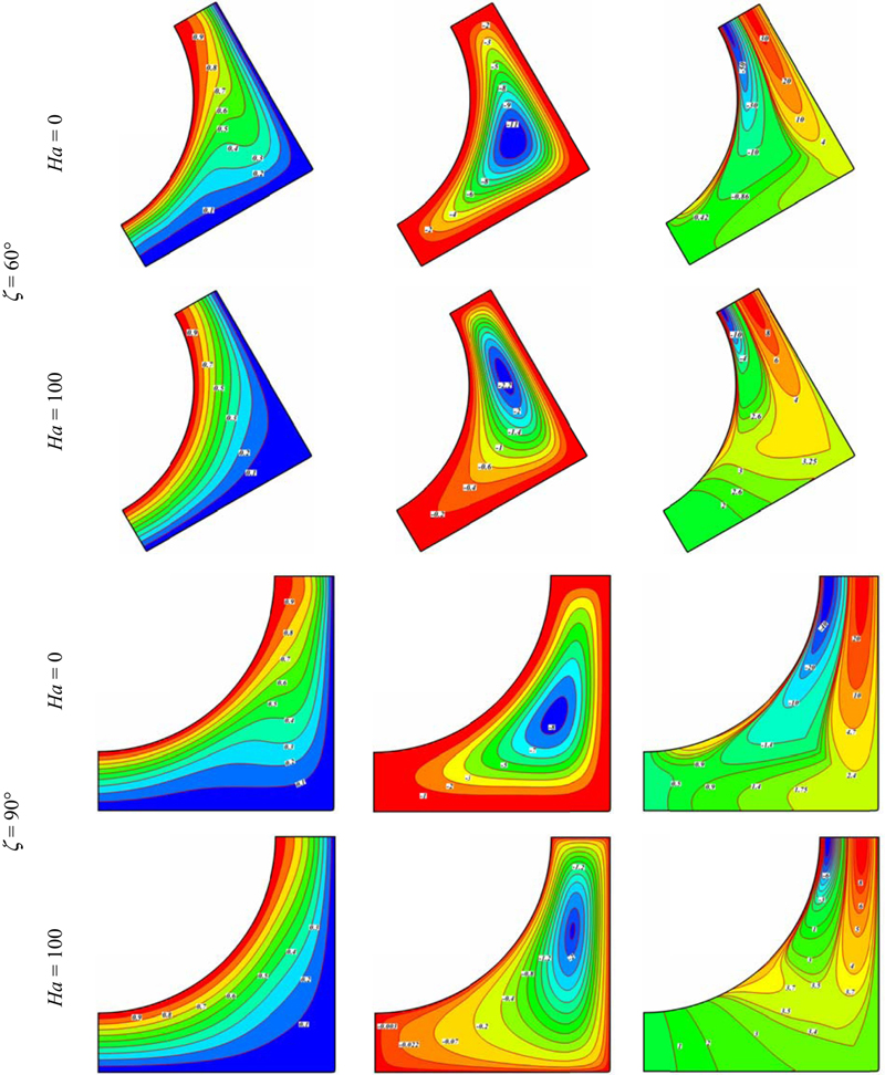
Figure 6.27 Comparison of the isotherms, streamlines, and heatlines for different values of Hartmann number and inclination angle at Ra = 105, φ = 0.04, and Pr = 6.2.
When the magnetic field is imposed on the enclosure, the velocity field suppressed owing to the retarding effect of the Lorenz force. So, intensity of convection weakens significantly. The braking effect of the magnetic field is observed from the maximum stream function value. The core vortex is shift upward vertically as the Hartmann number increases. Also, imposing magnetic field leads to omit the thermal plume over the inner wall. At high Hartmann number, the conduction heat transfer mechanism is more pronounced. For this reason, the isotherms are parallel to each other.
The heat flow within the enclosure is displayed using the heat function obtained from conductive heat fluxes (∂Θ/∂X, ∂Θ/∂Y) as well as convective heat fluxes (VΘ, UΘ). Heatlines emanate from hot regimes and end on cold regimes, illustrating the path of heat flow. The domination of conduction heat transfer in low Rayleigh number and high Hartmann number can be observed from the heatline patterns because no passive area exists. The increase of Ra causes the clustering of heatlines from hot to the cold wall, and generates passive heat transfer area in which heat is rotated without having significant effect on heat transfer between walls.
Fig. 6.28 shows the distribution of local Nusselt numbers along the surface of the inner circular wall for different inclination angle, Rayleigh number, and Hartmann number. Increasing Rayleigh number leads to an increase in local Nusselt number, but increasing Hartmann number and inclination angle cause local Nusselt number to decrease. At Ra = 103, because of domination conduction heat transfer mechanism, the distribution of the local Nusselt numbers along the surface of inner circular shows the symmetric shape. It is interesting to notice that at high Rayleigh number the local Nusselt number profiles are more complex due to the presence of thermal plume. In all cases expect for Ra = 105, γ = −90°, one minimum point exist in local Nusselt number profile which is occurred in lower values of |γ| with the increase of Hartmann number. Effects of Rayleigh number, Hartmann number, and inclination angle on average Nusselt number are shown in Fig. 6.29. Nusselt number is an increasing function of Rayleigh number, but it is a decreasing function of Hartmann number and inclined angle. Also, it can be found that effect of Hartmann number on Nusselt number is more pronounced at ζ = 0°.
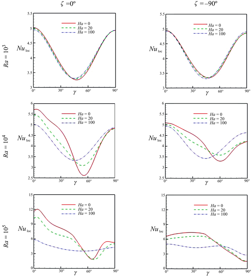
Figure 6.28 Effects of the Hartmann number, Rayleigh number, and inclination angle for Cu–water nanofluids on local Nusselt number.
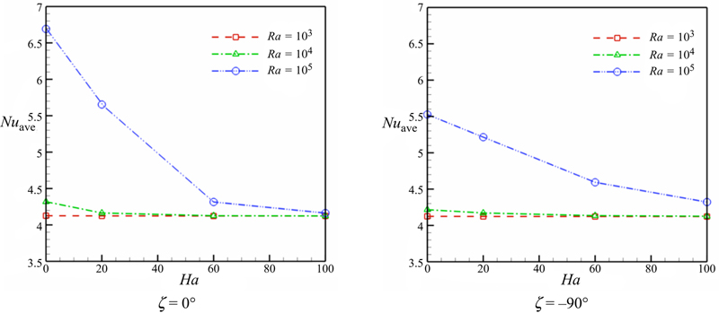
Figure 6.29 Effects of Rayleigh number, Hartmann number, and inclination angle on average Nusselt number at φ = 0.04.
The heat transfer enhancement ratio due to addition of nanoparticles for different values of ζ, Ha, and Ra is shown in Fig. 6.30. In general, it can be found that the effect of nanoparticles is more pronounced at low Rayleigh number and high values of Hartmann number because of the greater enhancement rate. This observation can be explained by noting that at low Rayleigh number the heat transfer is dominant by conduction. Therefore, the addition of high thermal conductivity nanoparticles will increase the conduction and make the enhancement more effective. Inclination angle has no significant effect on rate on enhancement when Ra = 103 and 104, while E increases with the increase of |ζ| when Ra = 105. Finally, the corresponding polynomial representation of such model for each of Nusselt number and rate of enhancement are presented as follows:
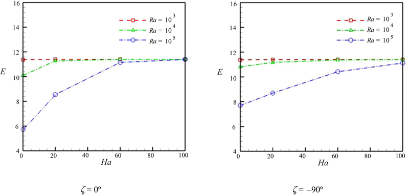
Figure 6.30 Effects of Rayleigh number, Hartmann number, and inclination angle on ratio of heat transfer enhancement due to addition of nanoparticles.
 (6.79)
 (6.80)
..................Content has been hidden....................
You can't read the all page of ebook, please click here login for view all page.