9.3. Heated permeable stretching surface in a porous medium using Nanofluid
9.3.1. Problem definition
Consider the steady, two-dimensional flow of a nanofluid near the stagnation point on a stretching sheet saturated at a porous surface (highly permeable) as shown in Fig. 9.14[21]. The stretching velocity Uw(x) and the free stream velocity U∞(x) are assumed to vary proportional to the distance x from the stagnation point, that is, Uw(x) = ax and U∞(x) = bx, where a and b are constants with a > 0 and b ≥ 0. It is assumed that the temperature at the stretching surface takes the constant values Tw, while the temperature of the ambient nanofluid, attained as y tends to infinity, takes the constant values T∞. The fluid is a water-based nanofluid containing different types of nanoparticles: Cu, Al2O3, Ag, and TiO2. It is assumed that the base fluid and the nanoparticles are in thermal equilibrium and no slip occurs between them.
Figure 9.14Figure of geometery.
Under these assumptions:
∂u∂x+∂υ∂y=0,
(9.114)
ρnf(u∂u∂x+υ∂u∂y−U∞dU∞dx)=μnf∂2u∂y2+μnfK(U∞−u),
(9.115)
(ρCp)nf(u∂T∂x+υ∂T∂y)=∂∂y(k∗nf∂T∂y),k∗nf=knf(1+ɛθ)
(9.116)
Subject to the boundary conditions
y=0:u=Uw(x),v=vw,T=Twy→∞:u→U∞(x),T→T∞
(9.117)
where u and υ are the velocity components along the x and y axes, respectively, T is fluid temperature, ɛ is thermal conductivity parameter and K is the permeability of the porous medium. Also, vw is the wall mass flux with vw < 0 for suctions and vw > 0 for injection, respectively.
The effective density ρnf, the effective dynamic viscosity μnf, the heat capacitance (ρCp)nf and the are given as:
ρnf=ρf(1−φ)+ρsφ
(9.118)
μnf=μf(1−φ)2.5
(9.119)
(ρCp)nf=(ρCp)f(1−φ)+(ρCp)sφ
(9.120)
Effective thermal conductivity (knf) can be incorporated from the following expression [21]:
knfkf=ks+(n−1)kf−(n−1)φ(kf−ks)ks+(n−1)kf+φ(kf−ks)
(9.121)
where n is the empirical shape factor for the nanoparticle. In particular, n = 3 for spherical shaped nanoparticles and n = 3/2 for cylindrical ones. Models of nanofluid based on different formulas for thermal conductivity and dynamic viscosity is shown in Table 9.5.
Table 9.5
Models of nanofluid based on different formulas for thermal conductivity and dynamic viscosity
Model
Shape of nanoparticles
Thermal conductivity
Dynamic viscosity
I
Spherical
knfkf=ks+2kf−2φ(kf−ks)ks+2kf+φ(kf−ks)
μnf=μf(1−φ)2.5
II
Cylindrical (nanotubes)
knfkf=ks+(1/2)kf−(1/2)φ(kf−ks)ks+(1/2)kf+φ(kf−ks)
μnf=μf(1−φ)2.5
The continuity equation (9.114) is satisfied by introducing a stream function ψ such that
u=∂ψ∂yandυ=−∂ψ∂x
(9.122)
The momentum and energy equations can be transformed into the corresponding ordinary differential equations by the following transformation:
η=(aυ)1/2y,f(η)=ψ(aυ)1/2x,θ(η)=T−T∞Tw−T∞
(9.123)
Using model I, the transformed ordinary differential equations are:
f′′′+ff′′−f′2+λ2+K1A1.(1−φ)2.5(λ−f′)=0,
(9.124)
1Pr⋅A1⋅A3⋅(1−φ)2.5A2((1+ɛθ)θ′′+ɛ(θ′)2)+fθ′=0.
(9.125)
subject to the boundary conditions (4) which become
f(0)=−vw(aυ)0.5=γ,f′(0)=1,θ(0)=1,f′(∞)→λ,θ(∞)→0.
(9.126)
Here prime denote differentiation with respect to η, λ = b/a is the Velocity ratio parameter, Pr=(μf(ρCp)f)/(ρfkf) is the Prandtl number and K1 = μf/(ρfKa) is the Permeability parameter and A1, A2, A3 are parameters having the following form:
A1=(1−φ)+ρsρfφ
(9.127)
A2=(1−φ)+(ρCp)s(ρCp)fφ
(9.128)
A3=knfkf=ks+2kf−2ϕ(kf−ks)ks+2kf+ϕ(kf−ks)
(9.129)
The quantities of practical interest in this study are the skin friction coefficient (Cf) and the local Nusselt number (Nux), which are defined as
Cf=μnfρfU2w(∂u∂y)y=0,Nu=xknfkf(Tw−T∞)(−∂T∂y)y=0,
(9.130)
with knf being the thermal conductivity of the nanofluid.
Therefore, the skin friction coefficient and the local Nusselt number can be expressed as
where Rex = ρfUwx/μf is the local Reynolds number based on the stretching velocity. The quantities C˜f and N˜ux are referred as the reduced skin friction coefficient and reduced local Nusselt number, respectively.
9.3.2. Effects of active parameters
The ordinary differential equations with the boundary conditions have been solved numerically for some values of the governing parameters. Thermal conductivity parameter, volume fraction of the nanoparticles, permeability parameter, suction/injection parameter, velocity ratio parameter, and different kinds of nanoparticles using the fourth order Runge–Kutta.
Effects of Thermal conductivity parameter (ɛ) and nanoparticle volume fraction (φ) on Temperature distribution and Nusselt number when K1 = 0.1 and Pr = 6.2 is shown in Fig. 9.15. Because of increasing in the thermal conductivity due to increase in ɛ, the thermal boundary layer thickness increases, thus decreases heat transfer rate at the surface. When the volume fraction of the nanoparticles increases from 0 to 0.2, the thermal boundary layer is increased. This agrees with the physical behavior in that when the volume fraction of copper increases the thermal conductivity increases, and then the thermal boundary layer thickness increases, hence increases heat transfer rate at the surface.
Figure 9.15Effect of Thermal conductivity parameter (ɛ) and nanoparticle volume fraction (φ) on Temperature distribution and Nusselt number when K1 = 0.1 and Pr = 6.2.
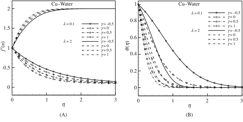
Fig. 9.16 graphical representation of the effect of the suction/injection parameter (γ) for Cu–Water on Velocity profile and Temperature distribution for two different values of Velocity ratio parameter (λ = 0.1 and λ = 2, when K1 = 0.1, φ = 0.1, ɛ = 0.1, and Pr = 6.2. We know that the effect of suction is to bring the fluid closer to the surface and, therefore, to reduce the thermal boundary layer thickness and in turn increases the Nusselt number, but opposite trend is observed for injection. When stronger injection is provided, the heated Cu–Water is pushed less from the wall than for a regular fluid (φ = 0), that is, the existence of the nanoparticle leads to a small increase of the velocity profiles, but for suction, it is noted an opposite behavior. It is clear that the thermal boundary layer thickness for the injection case is greater than for suction. When λ > 1, the flow has a boundary layer structure and when λ < 1 the flow has an inverted boundary layer structure, which results from the fact that when (b/a) < 1, the stretching velocity ax of the surface exceeds the velocity bx of the external stream. It is to be noted that no momentum boundary layer is formed when λ = 1. It is seen from Fig. 9.16, the thermal boundary layer thickness for λ < 1 is greater than for λ > 1. For λ = 0.1, the effect of suction is to decrease the velocity profile, whereas the effect of injection is to increase this profile. Also it can be found that for both cases, all boundary layer thicknesses increase with increasing values of suction/injection parameter.
Figure 9.16Effect of Suction or injection parameter (γ) and nanoparticle volume fraction (φ) on Velocity profile and Temperature distribution when K1 = 0.1, φ = 0.1, ɛ = 0.1, and Pr = 6.2.
Table 9.6 shows that the effects of permeability parameter (K1), suction/injection parameter (γ), velocity ratio parameter (λ), and nanoparticle volume fraction (φ) on skin friction coefficient when ɛ = 0.1 and Pr = 6.2. Physically, negative sign of C˜f implies that the stretching tube exerts a dragging force on the fluid and positive sign implies the opposite. For both suction(γ > 0) or injection (γ < 0) and both cases of λ (λ = 0.1 or λ = 2) it can be seen that the absolute values of skin friction increases due to increase in Permeability parameter and Suction/injection parameter, while it decreases due to decrease in nanoparticle volume fraction.
Table 9.6
Effects of Permeability parameter, Suction/injection parameter, Velocity ratio parameter, and nanoparticle volume fraction on skin friction coefficient when ɛ = 0.1 and Pr = 6.2 for Cu–Water
λ = 0.1
λ = 2
φ
K1
γ
0
0.05
0.1
0
0.05
0.1
0.1
−0.5
−0.80524
−0.79792
−0.79443
1.778452
1.773849
1.771663
0.1
0
−1.01007
−1.00264
−0.9991
2.041795
2.037279
2.035133
0.1
0.5
−1.26387
−1.25665
−1.25322
2.333717
2.329335
2.327254
0.5
0.5
−1.40827
−1.37611
−1.36056
2.425567
2.404448
2.394366
1
0.5
−1.5677
−1.5104
−1.48234
2.535495
2.495021
2.475585
0.5
−0.5
−0.95151
−0.91898
−0.90323
1.874645
1.852573
1.842026
1
−0.5
−1.11245
−1.05467
−1.02635
1.989145
1.947061
1.926822
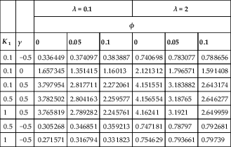
Table 9.7 shows that the effects of Permeability parameter (K1), Suction/injection parameter (γ), Velocity ratio parameter (λ) and nanoparticle volume fraction (φ) on Nusselt number when ɛ = 0.1 and Pr = 6.2 for Cu–Water. When λ = 0.1 and λ = 2, for suction Nusselt number decreases with increasing in nanoparticle volume fraction, whereas the opposite trend is observed for injection. For both suction or injection, Nusselt number increases due to increase the Permeability parameter when λ = 2, but opposite behavior is noted when λ = 0.1. However, increasing in γ leads to increase in Nusselt number for both the cases of λ.
Table 9.7
Effects of Permeability parameter, Suction/injection parameter, and nanoparticle volume fraction on Nusselt number when ɛ = 0.1 and Pr = 6.2 for Cu–Water
λ = 0.1
λ = 2
φ
K1
γ
0
0.05
0.1
0
0.05
0.1
0.1
−0.5
0.336449
0.374097
0.383887
0.740698
0.783077
0.788656
0.1
0
1.657345
1.351415
1.16013
2.121312
1.796571
1.591408
0.1
0.5
3.797954
2.817711
2.272061
4.151551
3.183882
2.643174
0.5
0.5
3.782502
2.804163
2.259577
4.156554
3.18765
2.646277
1
0.5
3.765819
2.789282
2.245761
4.16241
3.1921
2.649959
0.5
−0.5
0.305268
0.346851
0.359213
0.747181
0.78797
0.792681
1
−0.5
0.271571
0.316794
0.331823
0.754629
0.793661
0.79739
Table 9.8 shows that the effects of Velocity ratio parameter (λ) and nanoparticle volume fraction (φ) on skin friction coefficient and Nusselt number when ɛ = 0.1, K1 = 0.1, and Pr = 6.2 for Cu–Water. For both suction (γ > 0) and injection (γ < 0), when λ < 1 absolute values of skin friction decreases with increasing in λ, while it increases when λ > 1. Also, for both suction and injection and any values of λ it can be found that Nusselt number increases as Velocity ratio parameter increases.
Table 9.8
Effects of velocity ratio parameter and nanoparticle volume fraction on skin friction coefficient and Nusselt number when ɛ = 0.1, K1 = 0.1, and Pr = 6.2 for Cu–Water
C˜f
N˜ux
φ
γ
λ
0
0.05
0.1
0
0.05
0.1
0.5
0.1
−1.26387
−1.25665
−1.25322
3.797954
2.817711
2.272061
0.2
−1.17913
−1.17312
−1.17025
3.810096
2.831477
2.287149
1.7
1.552826
1.54958
1.548038
4.089999
3.123066
2.583777
2
2.333717
2.329335
2.327254
4.151551
3.183882
2.643174
−0.5
0.1
−0.80524
−0.79792
−0.79443
0.336449
0.374097
0.383887
0.2
−0.76547
−0.75929
−0.75635
0.350128
0.38932
0.400184
1.7
1.165817
1.162405
1.160785
0.67334
0.717759
0.725932
2
1.778452
1.773849
1.771663
0.740698
0.783077
0.788656
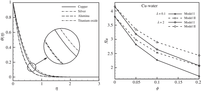
Table 9.9 shows variation in Nusselt number with different base fluids (Water Pr = 6.2 and Ethylene glycol Pr = 203.6) when K1 = 0.1, γ = 0.5, λ = 0.1. For fixed values of nanoparticle volume fraction, selecting Ethylene glycol instead of Water as base fluid lead to decrease thermal boundary layer thickness, so, Cu–Ethylene glycol has higher Nusselt number than Cu–Water due to lower thermal conductivity. Tables 9.10 and 9.11 display the behavior of the skin friction coefficient and Nusselt number using different nanofluids. Fig. 9.17 (A) shows that temperature distribution for different types of nanofluids when M = 1, S = 0.1, n = 1, λ = 0.1, φ = 0.1 and Pr = 6.2. These tables show that by using different types of nanofluid the value of C˜f, N˜ux and temperature profile change. This means that the nanofluids will be important in the cooling and heating processes. Choosing Titanium oxide as the nanoparticle leads to the maximum amount rate of hate transfer, while selecting Silver leads to the minimum amount of it. Also, choosing Alumina as the nanoparticle leads to the maximum amount skin friction coefficient, while selecting Silver leads to the minimum amount of it. In Fig. 9.17B, the Nusselt numbers versus the volume fraction of nanoparticle is shown when different models of nanofluid based on different formulas for thermal conductivity and dynamic viscosity is used. For all amount of λ, model II for nanotubes has higher Nusselt number than model I for spherical shaped nanoparticles due to lower thermal conductivity.
Table 9.9
Variation in Nusselt number with different base fluids (Water Pr = 6.2 and Ethylene glycol Pr = 203.6) when K1 = 0.1, γ = 0.5, λ = 0.1
Cu–Water
Cu–Ethylene glycol
φ
ɛ
0
0.05
0.1
0
0.05
0.1
0
4.138303
3.066625
2.470897
103.7016
76.98598
62.00115
0.1
3.797954
2.817711
2.272061
94.3584
70.06946
56.44514
0.5
2.883762
2.147712
1.735969
69.44076
51.62293
41.62623
1
2.245959
1.678457
1.359372
52.307
38.93695
31.43358
Table 9.10
Effects of the nanoparticle volume fraction for different types of nanofluids on skin friction coefficient when M = 1 and λ = 0.1
λ
φ
Nanoparticles
Cu
Ag
Al2O3
TiO2
0.1
0.05
−1.26387
−1.25498
−1.26346
−1.263
0.1
−1.25322
−1.25095
−1.26396
−1.26315
2
0.05
2.329335
2.328318
2.333467
2.333187
0.1
2.327254
2.325883
2.333774
2.333277
Table 9.11
Effects of the nanoparticle volume fraction for different types of nanofluids on Nusselt number when S = 0.1, n = 1, M = 1, λ = 0.1, and Pr = 6.2
λ
φ
Nanoparticles
Cu
Ag
Al2O3
TiO2
0.1
0.05
3.797954
2.668673
3.312571
3.329105
0.1
2.272061
2.082538
2.961854
2.995371
2
0.05
3.183882
3.036321
3.67321
3.689447
0.1
2.643174
2.45449
3.32729
3.36026
Figure 9.17(A) Temperature distribution for different types of nanofluids when K1 = 0.1, φ = 0.1, ɛ = 0.1, γ = 0.5, λ = 0.1, and Pr = 6.2; (B) Variation in Nusselt number with nanoparticle volume fraction for different models K1 = 0.1, ɛ = 0.1, γ = 0.5, and Pr = 6.2.
9.4. Two phase modeling of nanofluid in a rotating system with permeable sheet
9.4.1. Problem definition
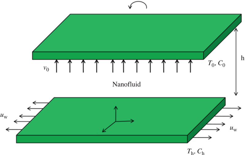
Consider the steady nanofluid flow between two horizontal parallel plates when the fluid and the plates rotate together around the y-axis which is normal to the plates with an angular velocity. A cartesian coordinate system is considered as follows: the x-axis is along the plate, the y-axis is perpendicular to it and the z-axis is normal to the x y plane (see Fig. 9.18) [22]. The upper plate is subjected to a constant wall injection velocity v0 (> 0), respectively. The plates are located at y = 0 and y = h. The lower plate is being stretched by two equal and opposite forces so that the position of the point (0,0,0) remains unchanged. The upper plate is subjected to a constant flow injection with a velocity v0.
Figure 9.18Geometry of problem.
The governing equations in a rotating frame of reference are:
Here u, v, and z are the velocities in the x, y, and z directions respectively. Also p* is the modified fluid pressure. The absence of ∂p*∂z in Eq. (9.135) implies that there is a net cross-flow along the z-axis. The relevant boundary conditions are:
Skin friction coefficient (Cf) along the stretching wall and Nusselt number (Nu) along the stretching wall are defined as
C˜f=(Rxh)Cf=f′′(0),Nu=−θ'(0)
(9.152)
9.4.2. Effects of active parameters
In this study, three dimensional two phase simulation of nanofluid flow and heat transfer is investigated. Fourth order Runge–Kutta integration scheme featuring a shooting technique with the MAPLE package is used to solve this problem.
Effect of injection parameter on velocity, temperature, concentration profiles is shown in Fig. 9.19. As injection parameter increases, velocity profiles increase. Temperature profile decreases with increase of injection parameter while opposite trend is observed for concentration profile.
Figure 9.19Effect of injection parameter on velocity profiles (f, g), temperature profile (θ), and concentration profile (θ) when Re = 0.5, Kr = 0.5, Sc = 0.5, Nb = Nt = 0.1, and Pr = 10.
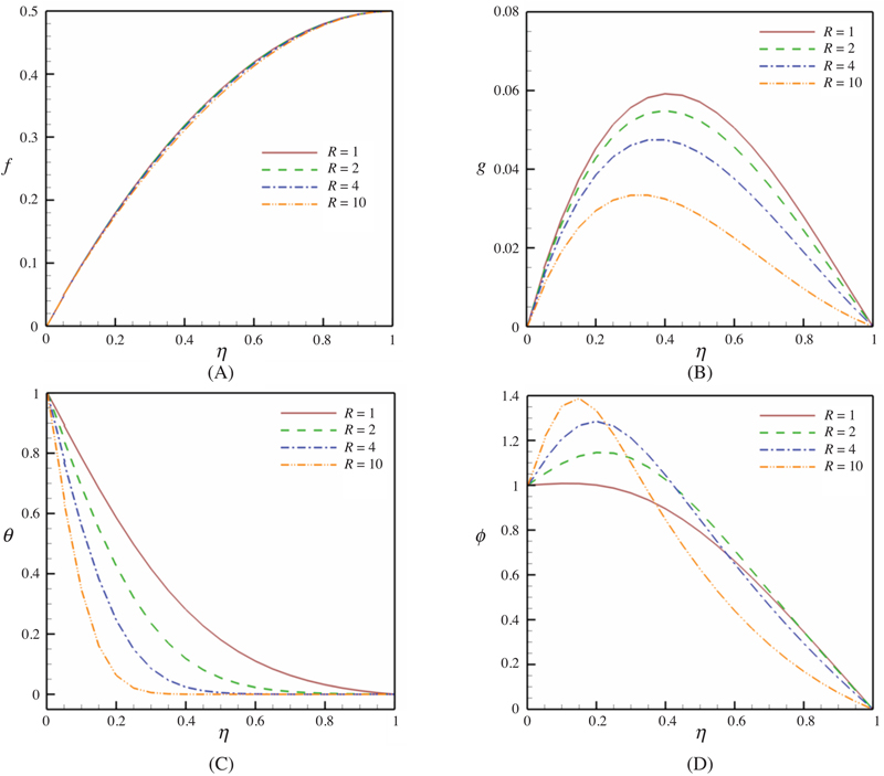
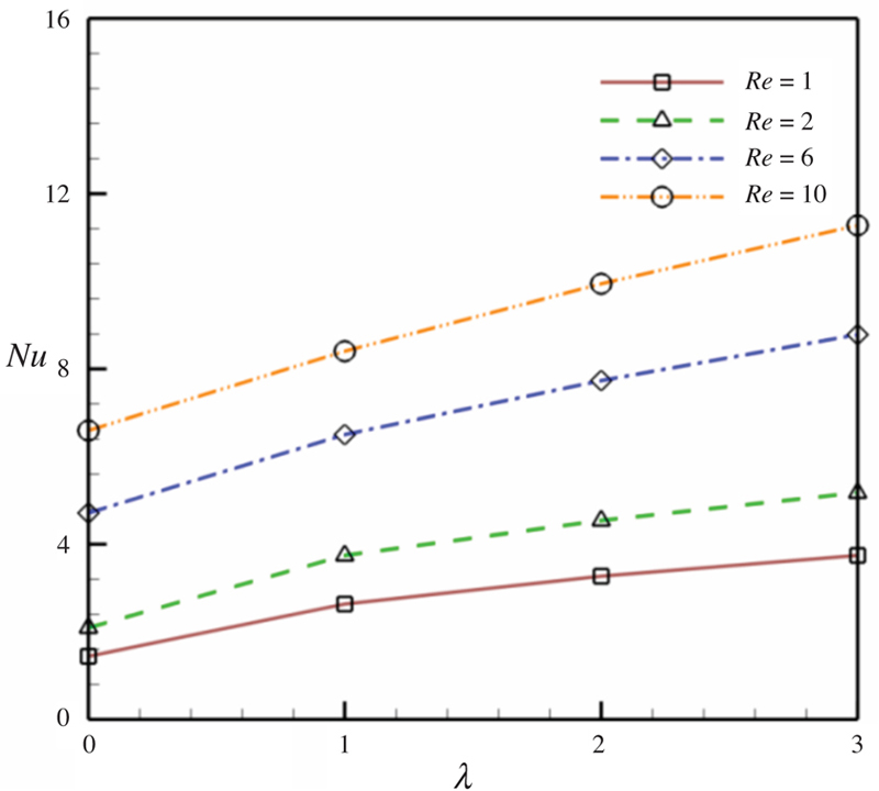
Fig. 9.20 shows the effects of Reynolds number on velocity, temperature, and concentration profiles. Effects of injection parameter and Reynolds number on Nusselt number is shown in Fig. 9.21. It is worth to mention that the Reynolds number indicates the relative significance of the inertia effect compared to the viscous effect. Thus, both velocity and temperature boundary layer thicknesses decrease with increase of Reynolds number and in turn increasing Reynolds number leads to increase in the magnitude of the skin friction coefficient and Nusselt number. Also it can be seen that concentration profile increases with augment of Reynolds number. Also it can be seen that Nusselt number increases with increase of injection parameter.
Figure 9.20Effect of Reynolds number on velocity profiles (f, g), temperature profile (θ), and concentration profile (φ) when λ = 0.5, Kr = 0.5, Sc = 0.5, Nb = Nt = 0.1, and Pr = 10.
Figure 9.21Effects of injection parameter and Reynolds number on Nusselt number when Kr = 0.5, Nt = 0.1, Nb = 0.1, Sc = 0.1, and Pr = 10.
Effects of Rotation parameter on velocity profile and Nusselt number are depicted in Fig. 9.22 and Table 9.12, respectively. With increasing Rotation parameter, the transverse velocity increases. As Rotation parameter increases thermal boundary layer thickness decreases and in turn Nusselt number increases with increase of Kr.
Figure 9.22Effect of Rotation parameter on velocity profile when Re = 0.5, λ = 0.5, Sc = 0.5, Nb = Nt = 0.1.
Table 9.12
Effect of Rotation parameter on Nusselt number when Nt = 0.1, Nb = 0.1, Sc = 0.1, Re = 1
λ
Kr
0.5
2
4
6
1
2.633504
2.633507
2.633518
2.634296
2
3.271111
3.271753
3.274186
3.279422
3
3.745806
3.746079
3.747427
3.751176
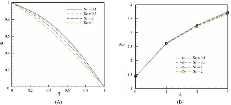
Fig. 9.23 shows the effect of Schmidt number on concentration profile and Nusselt number. Schmidt number is a dimensionless number defined as the ratio of momentum diffusivity (viscosity) and mass diffusivity. So concentration profile decreases as Schmidt number increases. Also it can be concluded that increasing Schmidt number causes a slight decrease in rate of heat transfer.
Figure 9.23Effect of Schmidt number on concentration profile and Nusselt number when (A) Re = 0.5, λ = 0.5, Kr = 0.5, Nb = Nt = 0.1; (B) Kr = 0.5, Nt = 0.1, Nb = 0.1, Re = 1, and Pr = 10.
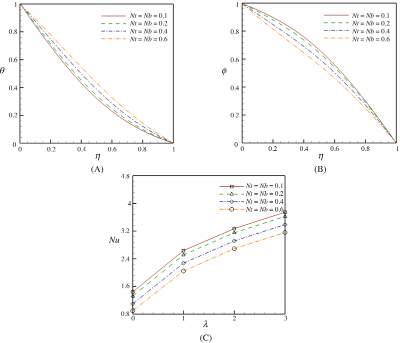
Effects of Brownian parameter and thermophoretic parameter on temperature, concentration profiles and Nusselt number are shown in Fig. 9.24. These active parameters have similar effects on heat and mass transfer characteristics. It means that temperature boundary layer thickness increases with increase of them while opposite trend is observed for concentration boundary layer thickness. Nusselt number is a decreasing function of Thermophoretic parameter and Brownian parameter.
Figure 9.24Effects of Brownian parameter and thermophoretic parameter on temperature, concentration profile, and Nusselt number when (A, B) Re = 0.5, λ = 0.5, Kr = 0.5, Sc = 0.5; and (C) Kr = 0.5, Sc = 0.1, Re = 1, and Pr = 10.
9.5. KKL correlation for simulation of nanofluid flow and heat transfer in a permeable channel
9.5.1. Problem definition
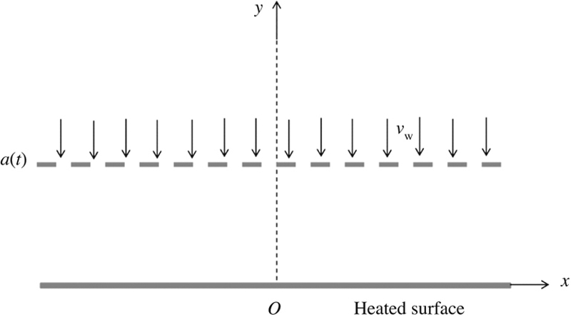
The unsteady flow between two parallel flat plates is considered as shown in Fig. 9.25[23]. The wall, which coincides with the x-axis, is stationary and heated externally. In order to cool the heated wall, cooled fluid is injected with velocity vw uniformly from the other plate, which expands or contracts at a time-dependent rate a(t). Take y to be perpendicular to the plates and assume u and v to be the velocity components in the x and y directions respectively. In this perspective the flow field may be assumed to be stagnation flow. The nanofluid is a two component mixture with the following assumptions: incompressible; no-chemical reaction; negligible radiative heat transfer; nanosolid particles and the base fluid are in thermal equilibrium and no slip occurs between them. Under these assumptions, the Navier–Stokes equations are:
Figure 9.25Geometry of problem.
∂u∂x+∂v∂y=0,
(9.153)
ρnf(∂u∂t+u∂u∂v+v∂u∂y)=−∂p∂x+μnf(∂2u∂x2+∂2u∂y2),
(9.154)
ρnf(∂v∂t+u∂v∂v+v∂v∂y)=−∂p∂y+μnf(∂2v∂x2+∂2v∂y2),
(9.155)
∂T∂t+u∂T∂x+v∂T∂y=knf(ρCp)nf(∂2T∂x2+∂2T∂y2).
(9.156)
Here u and v are the velocities in the x and y directions respectively, T is the temperature, P is the pressure, effective density ρnf and the effective heat capacity (ρCp)nf of the nanofluid are defined as:
ρnf=(1−φ)ρf+φρp(ρCp)nf=(1−φ)(ρCp)f+φ(ρCp)p
(9.157)
(knf) and (μnf) are obtained according to Koo–Kleinstreuer–Li (KKL) model [24]:
Thermo physical properties of water and nanoparticles [24]
ρ (kg/m3)
Cp (J/kg·K)
k (W/m·K)
dp (nm)
Pure water
997.1
4179
0.613
—
Al2O3
3970
765
25
47
Table 9.14
The coefficient values of Al2O3–Water nanofluids [24]
Coefficient values
Al2O3–Water
a1
52.813488759
a2
6.115637295
a3
0.6955745084
a4
4.17455552786E-02
a5
0.176919300241
a6
−298.19819084
a7
−34.532716906
a8
−3.9225289283
a9
−0.2354329626
a10
−0.999063481
The relevant boundary conditions are:
u=0,v=−vw=−Aa∙,T(a)=T0aty=a(t),u=0,v=0;aty=0.
(9.160)
where A=v/wa∙ is the measure of wall permeability, and T0 is the temperature of the porous plate (y = a) which has the same temperature as that of the incoming coolant.
Introducing the stream function
ψ=vxaF(η,t),
(9.161)
where η = y/a.
Substituting ψ into Eqs. (9.153)–(9.155) and eliminating the pressure term from the momentum equation, the following expression can be obtained:
Note that the expansion ratio will be positive for expansion and negative for contraction.
α=aa∙υf
(9.164)
And A1 and A2 are constant parameters that are defined as:
A1=ρnfρf,A2=μnfμf,
(9.165)
The boundary conditions are
Fη(0)=0,F(0)=0,Fη(1)=0,F(1)=A1A2R,
(9.166)
where Re is the Reynolds number defined by Re = avw/υf. Note that Re is positive for injection and negative for suction. For this model, we only consider the case that Re is positive.
Let
f=FR,l=xa
(9.167)
A similar solution with respect to both space and time can be developed following the transformation [25,26]. This can be accomplished by considering in the case: α is a constant and f = f (η). It leads to fηηt = 0. To realize this condition, the value of expansion ratio α must be specified by its initial value
α=aa∙υf=a0a0∙υf=cte,
(9.168)
where a0 and a0∙ denote the initial channel height and expansion ratio, respectively. Integrating Eq. (9.168) with respect to time, the similar solution can be achieved. The result is
aa0=1+2υfαta−20−−−−−−−−−−√
(9.169)
For a physical setting in which the injection coefficient A is constant [26]. Since vw=Aa∙, an expression for the injection velocity variation can be determined. From Eqs. (9.168) and (9.169), it is clear that
At a distance η form the wall, the temperature of the fluid can be expressed as:
T=T0+∑Cm(xa)mqm(0)
(9.173)
and the temperature of the heated wall can be expressed as:
A3A4(−αPr(mqm+ηqm′)+PrR(mf′qm−fqm′))=qm′′
(9.174)
Where A3 and A4 are constant parameters that are defined as:
A3=(ρCp)nf(ρCp)f,A4=knfkf
(9.175)
with boundary conditions
qm(0)=1,qm(1)=0
(9.176)
However, it is not possible to get a single value for the heat transfer coefficient along the heated wall if the wall temperature follows a polynomial variation, unless the temperature along the heated surface is expressed by a single term in Eq. (9.173), that is,
Tw=T0+Cm(xa)mqm(0)
(9.177)
In this case the nondimensional Nusselt number is obtained as:
Nu=−knfkf∂T∂η/(Tw−T0)=−qm′(0)
(9.178)
9.5.2. Numerical method
Before employing the Runge–Kutta integration scheme, first we reduce the governing differential equations into a set of first order ODEs [27,28].
Let x1=η,x2=f,x3=f′,x4=f′′,x5=f′′′,x6=qm,x7=qm′. We obtain the following system:
The previous nonlinear coupled ODEs along with initial conditions are solved using fourth Order Runge-Kutta integration technique. Suitable values of the unknown initial conditions u1, u2, u3, and u4 are approximated through Newton’s method until the boundary conditions at f′(1)=0,f(1)=1,qm(1)=0 are satisfied. The computations have been performed by using MAPLE. The maximum value of x = 1, to each group of parameters is determined when the values of unknown boundary conditions at x = 0 do not change to a successful loop with error less than 10–6. Recently, researchers utilized new numerical methods for simulating nanofluid flow and heat transfer [29–41].
9.5.3. Effects of active parameters
Flow and heat transfer of nanofluid fluid between two parallel plates is studied numerically. One of plates is externally heated, and the other plate, through which coolant fluid is injected, expands or contracts with time. Effect of Reynolds number and expansion ratio on the velocity profiles is shown in Fig. 9.26. As expansion ratio increases f increases. This figure shows that there is a maximum point for f’ between the two plates. Increasing expansion ratio leads to shift maximum velocity point of f’ to the solid wall. Also it can be seen that maximum values of f’ increases with increase of expansion ratio. Effect of Reynolds number on velocity profiles is similar to expansion ratio.
Figure 9.26Effect of Reynolds number and expansion ratio on the velocity profiles at (A) φ = 0.04, Re = 1 and (B) φ = 0.04, α = 1.
Fig. 9.27 shows the effect of volume fraction of nanofluid on the temperature profile. The sensitivity of thermal boundary layer thickness to volume fraction of nanoparticles is related to the increased thermal conductivity of the nanofluid. In fact, higher values of thermal conductivity are accompanied by higher values of thermal diffusivity. The high values of thermal diffusivity cause a fall in the temperature gradients and accordingly increase the boundary thickness. This increase in thermal boundary layer thickness reduces the Nusselt number; however, the Nusselt number is a multiplication of temperature gradient and the thermal conductivity ratio (conductivity of the nanofluid to the conductivity of the base fluid). Since the reduction in temperature gradient due to the presence of nanoparticles is much smaller than thermal conductivity ratio therefore an enhancement in Nusselt is taken place by increasing the volume fraction of nanoparticles.
Figure 9.27Effect of volume fraction of nanofluid on the temperature profile when α = 1, Re = 1, m = 1, and Pr = 6.2.
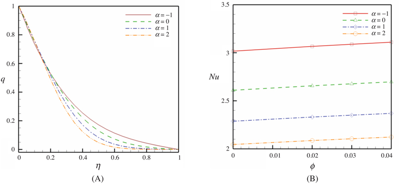
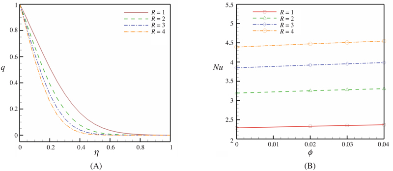
Fig. 9.28 demonstrates the effect of expansion ratio on temperature profile and Nusselt number. Increasing expansion ratio causes thermal boundary layer thickness to increase; therefore Nusselt number decreases with increase of expansion ratio. Effect of Reynolds number on temperature profile and Nusselt number is shown in Fig. 9.29. Reynolds number indicates the relative significance of the inertia effect compared to the viscous effect. Thus, thermal boundary layer thickness decreases as Re increases and in turn increasing Reynolds number leads to increase in Nusselt number. Fig. 9.30 shows the effect of power law index on temperature profile and Nusselt number. Temperature gradients near the solid wall increases with augment of power law index. So Nusselt number is an increasing function of power law index.
Figure 9.28Effect of expansion ratio on (A) the temperature profile when Re = 1, m = 1, φ = 0.04 and (B) Nusselt number when Re = 1, m = 1, and Pr = 6.2.
Figure 9.29Effect of Reynolds number on (A) the temperature profile when α = 1, m = 1, φ = 0.04 and (B) Nusselt number when α = 1, m = 1, and Pr = 6.2.
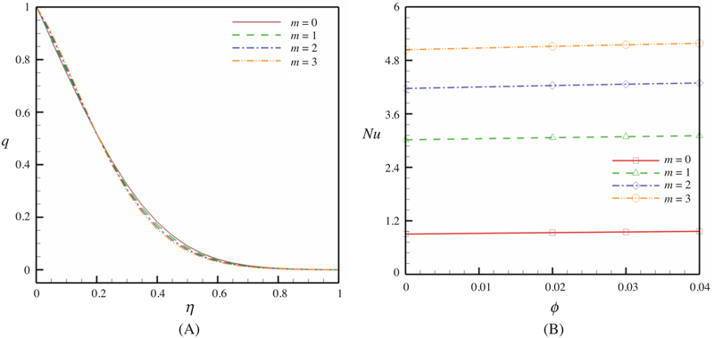
Figure 9.30Effect of power law index on (A) the temperature profile when α = 1, Re = 1, φ = 0.04 and (B) Nusselt number when α = 1, Re = 1, and Pr = 6.2.
The enhancement of heat transfer between the case of φ = 0.04 and the pure fluid (base fluid) case is defined as:
E=Nu(φ=0.04)−Nu(basefluid)Nu(basefluid)×100
(9.181)
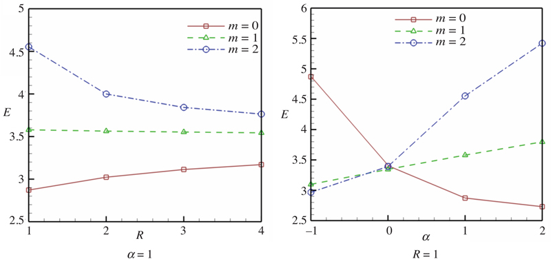
Heat transfer enhancement due to addition of nanoparticles for different values of Reynolds number, expansion ratio and power law index is shown in Fig. 9.31. When m = 0, enhancement of heat transfer increases as Reynolds number increases but it decrease with increase of Re when m > 0. Also values of enhancement for m > 0 are greater than m = 0. The enhancement of heat transfer increases with augment of expansion ratio when m > 0 but opposite trend is observed for m = 0. It is interesting observation that for all values of power law index, values of E has no significant changes when α = 0.
Figure 9.31Effects of the Reynolds number, expansion ratio, and power law index on enhancement heat transfer when Pr = 6.2.


 (9.114)
 (9.115)
 (9.116)
 (9.117)
 (9.119)
 (9.121)

 (9.122)
 (9.123)
 (9.124)
 (9.125)
 (9.126)
 (9.127)
 (9.128)
 (9.129)
 (9.130)
 (9.131)
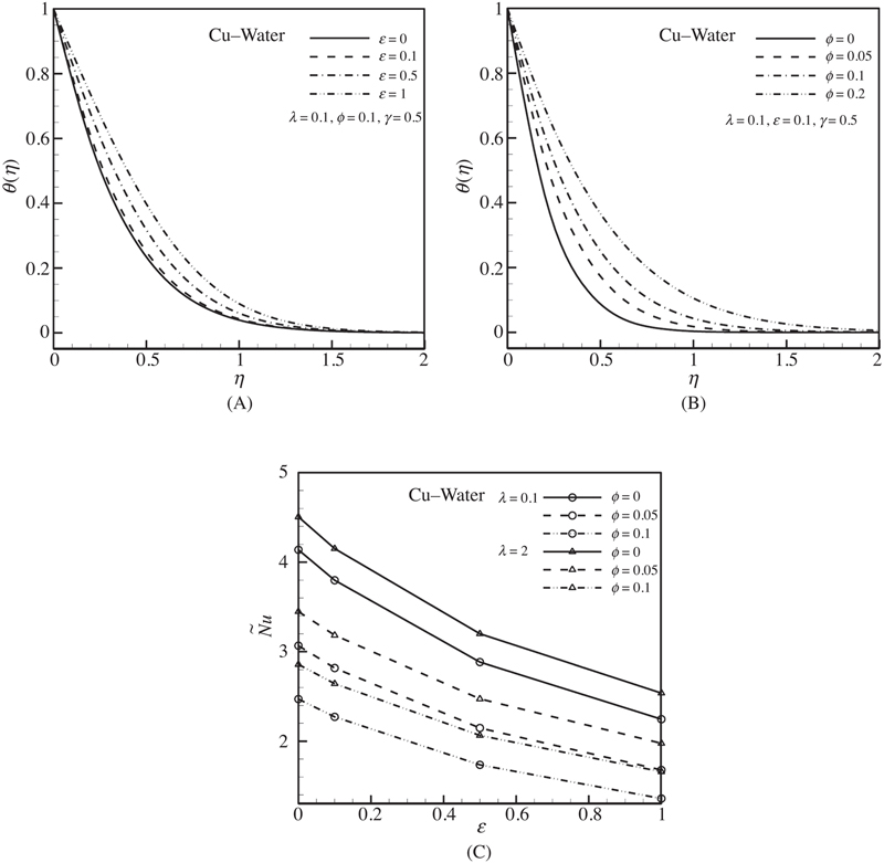


 (9.132)
 (9.133)
 (9.134)
 (9.135)
 (9.136)
 (9.137)
 in Eq. (9.135) implies that there is a net cross-flow along the z-axis. The relevant boundary conditions are:
 (9.138)
 (9.139)
 (9.140)
 (9.141)
 (9.143)
 (9.149)
 (9.150)
 (9.151)
 (9.152)
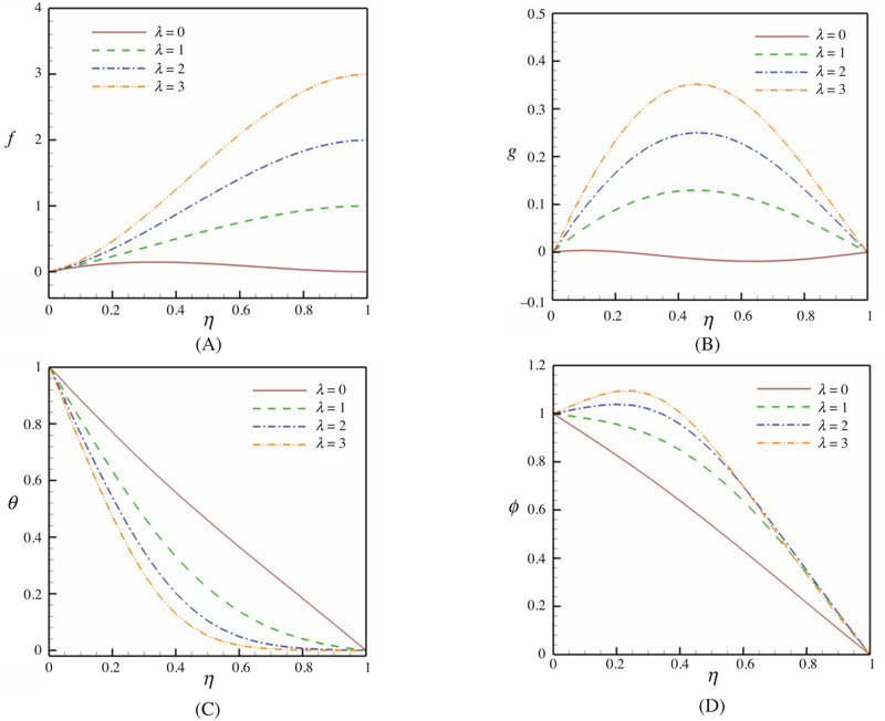


 (9.153)
 (9.154)
 (9.155)
 (9.156)
 (9.157)
 (9.158)
 (9.159)
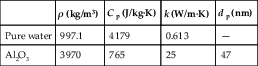
 (9.160)
 (9.161)
 (9.162)
 (9.163)
 (9.164)
 (9.165)
 (9.166)
 (9.167)
 (9.168)
 (9.169)
 (9.170)
 (9.171)
 (9.173)
 (9.174)
 (9.175)
 (9.177)
 (9.178)
 (9.179)
 (9.180)
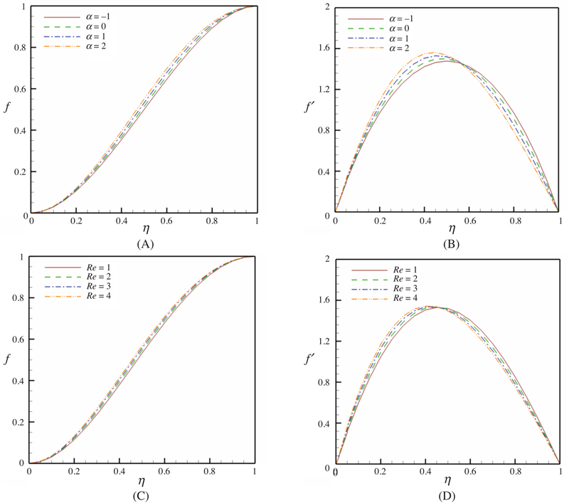

 (9.181)