
Chapter 4
Nanofluid Flow and Heat Transfer in the Presence of Thermal Radiation
Abstract
The thermal radiation has an important role in the overall surface heat transfer when the convection heat transfer coefficient is small. It is well known that the effect of thermal radiation is important in space technology and high temperature processes. Thermal radiation also plays an important role in controlling heat transfer process in polymer processing industry. In this chapter, nanofluid hydrothermal behavior in the presence of thermal radiation is investigated.
Keywords
thermal radiation
nanofluid
viscous dissipation
Brownian
thermophoresis
4.1. MHD free convection of Al2O3–water nanofluid considering thermal radiation
4.1.1. Problem definition
The numerical model consists in a two-dimensional square cavity with side equal to L which represents the characteristic dimension of the problem (Fig. 4.1A) [1]. The heat source is centrally located on the bottom surface and its length L/3. The cooling is achieved by the two vertical walls. The heat source has constant heat flux q″, while the cooling walls have a constant temperature Tc; all the other surfaces are adiabatic. Also, it is also assumed that the uniform magnetic field  of constant magnitude
  is applied, where
  and
and  are unit vectors in the Cartesian coordinate system. The orientation of the magnetic field forms an angle θM with horizontal axis such that θM = cot−1 (Bx/By). The electric current J and the electromagnetic force F are defined by
  and
and  , respectively.
of constant magnitude is applied, where 
Figure 4.1 (A) Geometry and the boundary conditions; (B) a sample triangular element and its corresponding control volume.
The flow is steady, two-dimensional, laminar, and incompressible. The induced electric current and Joule heating are neglected. The magnetic Reynolds number is assumed to be small, so that the induced magnetic field can be neglected compared with the applied magnetic field. The Rosseland approximation is used to describe the radiative heat flux in the energy equation. The radiative heat flux in the x-direction is considered negligible in comparison with the y-direction. Neglecting displacement currents, induced magnetic field, and using the Boussinesq approximation, the governing equations of heat transfer and fluid flow for nanofluid can be obtained as follows:
 (4.1)
(4.1)
 (4.2)
(4.2)
 (4.3)
(4.3)
 (4.4)
(4.4)where the radiation heat flux qr is considered according to Rosseland approximation such that  where σ0 and βR are the Stefan–Boltzmann constant and the mean absorption coefficient, respectively. Following Raptis [2], the fluid-phase temperature differences within the flow are assumed to be sufficiently small, so that T4 may be expressed as a linear function of temperature. This is done by expanding T4 in a Taylor series about the temperature Tc and neglecting higher order terms to yield,
  .
.
where σ0 and βR are the Stefan–Boltzmann constant and the mean absorption coefficient, respectively. Following Raptis [2], the fluid-phase temperature differences within the flow are assumed to be sufficiently small, so that T4 may be expressed as a linear function of temperature. This is done by expanding T4 in a Taylor series about the temperature Tc and neglecting higher order terms to yield, The effective density, the thermal expansion coefficient, heat capacitance, and effective electrical conductivity of the nanofluid are defined as:
 (4.5)
(4.5)
 (4.6)
(4.6)
 (4.7)
(4.7)
 (4.8)
(4.8)The stream function and vorticity are defined as:
 (4.9)
(4.9)The stream function satisfies the continuity Eq. (4.1). The vorticity equation is obtained by eliminating the pressure between the two momentum equations, that is, by taking y-derivative of Eq. (4.2) and subtracting from it the x-derivative of Eq. (4.3). This gives:
 (4.10)
 (4.11)
 (4.12)
By introducing the following nondimensional variables:
 (4.13)
Using the dimensionless parameters, the equations now become:
 (4.14)
 (4.15)
 (4.16)
where Raf = gβfL4q″/(kf αf, υf) is the Rayleigh number for the base fluid,  is the Hartmann number, and Prf = υf/αf is the Prandtl number for the base fluid. Also,
  and
and  are radiation parameter and viscous dissipation parameter, respectively. The boundary conditions as shown in Fig. 4.1 are as follows:
 (4.17)
The values of vorticity on the boundary of the enclosure can be obtained using the stream function formulation and the known velocity conditions during the iterative solution procedure. The local Nusselt number of the nanofluid along the heat source can be expressed as:
 (4.18)
The average Nusselt number on hot circular wall is evaluated as:
 (4.19)
To estimate the enhancement of heat transfer between the case of  and the pure fluid (base fluid) case, the enhancement is defined as:
 (4.20)
4.1.2. Effects of active parameters
Effect of thermal radiation on the improvement of magnetohydrodynamic free convective heat transfer in a square cavity, which is heated by a constant flux heating element at the bottom surface, is investigated. CVFEM was utilized to obtain the numerical simulation. The enclosure is filled with Al2O3–water nanofluid. The effective thermal conductivity and viscosity of nanofluid are calculated by KKL correlation. Effect of active parameters, such as Rayleigh number (Ra = 103, 104, and 105), Hartmann number (Ha = 0, 20, 60, and 100), viscous dissipation parameter (ɛ = 0–0.03), radiation parameter (Rd = 0, 1, and 2), and volume fraction of nanoparticle (ɸ = 0 and 0.04) on flow and heat transfer are examined when Pr = 6.2.
The effects of radiation parameter, viscous dissipation parameter, Hartmann number, and Rayleigh number on isotherms and streamlines are depicted in Figs. 4.2–4.4. It is evident from this figure that the flow circulation increases with the increase of radiation parameter. Moreover, the streamlines begin to take the enclosure geometry. Also, it can be seen that isotherms move upward. As viscous dissipation parameter increases, ψmax increases and isotherms move away from bottom heater. By increasing Rayleigh number, the prominent heat transfer mechanism is turned from conduction to convection.

Figure 4.2 Effects radiation parameter, viscous dissipation parameter, Hartmann number of on isotherms (left), and streamlines (right) when ɸ = 0.04, Ra = 103.

Figure 4.3 Effects radiation parameter, viscous dissipation parameter, Hartmann number of on isotherms (left), and streamlines (right) when ɸ = 0.04, Ra = 104.
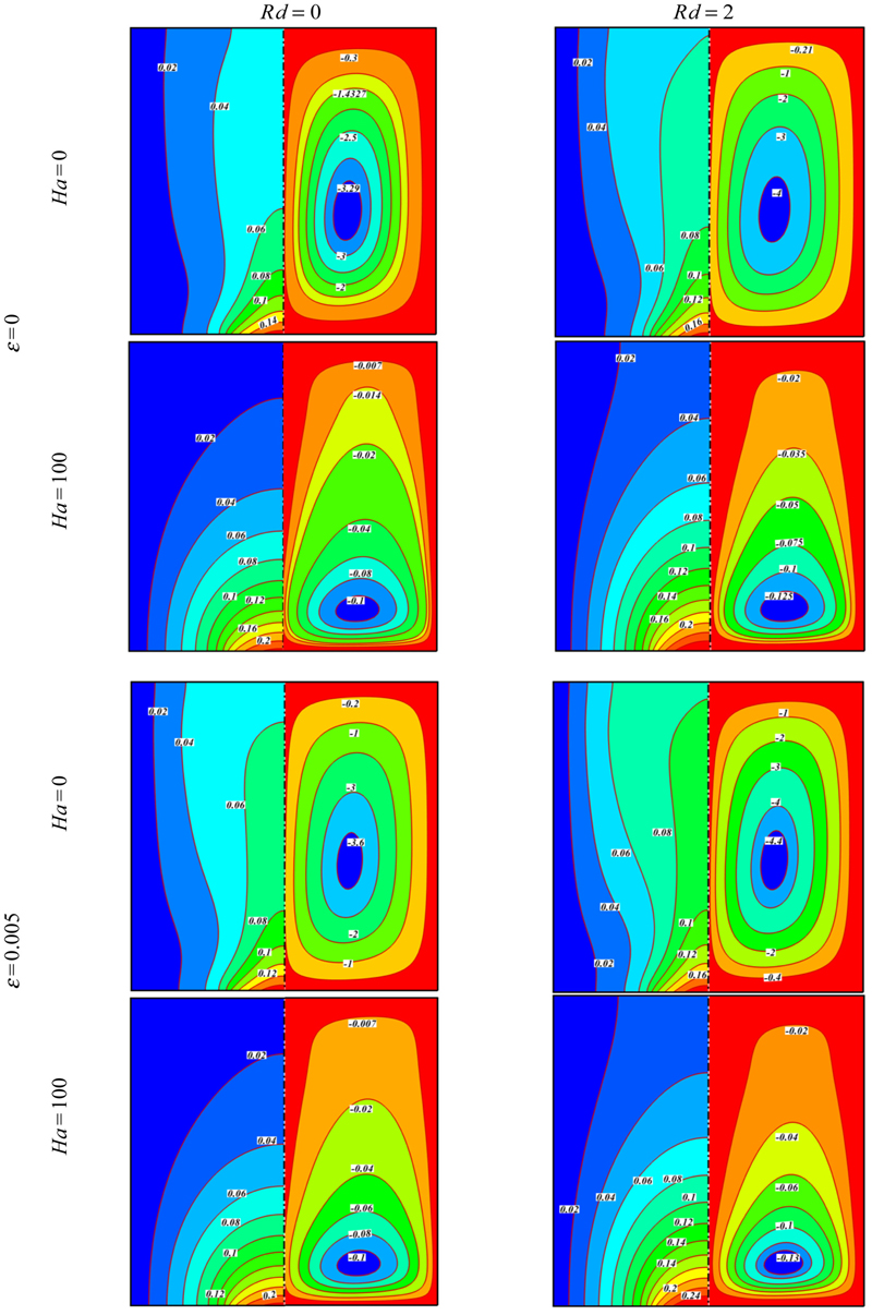
Figure 4.4 Effects of radiation parameter, viscous dissipation parameter, Hartmann number on isotherms (left), and streamlines (right) when ɸ = 0.04, Ra = 105.
When the magnetic field is imposed on the enclosure, the velocity field suppressed owing to the retarding effect of the Lorenz force. So, intensity of convection weakens significantly. The braking effect of the magnetic field is observed from the maximum stream function value. The core vortex is shift downward vertically as the Hartmann number increases. Also, imposing magnetic field leads to omit the thermal plume over the bottom wall. At high Hartmann number the conduction heat transfer mechanism is more pronounced. For this reason, the isotherms are parallel to each other.
The effects of radiation parameter, viscous dissipation parameter, Hartmann number, and Rayleigh number on average Nusselt number are shown in Fig. 4.5. Increasing Hartmann number causes Lorenz force to increase and leads to a substantial suppression of the convection. So, Nusselt number has reverse relationship with Hartmann number. Nusselt number increases with the augment of Rayleigh number due to domination of convective heat transfer. As radiation parameter increases, Nusselt number increases but the opposite trend is observed for viscous dissipation parameter.

Figure 4.5 Effects of radiation parameter, viscous dissipation parameter, Hartmann number, and Rayleigh number on average Nusselt number when ɸ = 0.04, Pr = 6.2.
Fig. 4.6 shows the effects of radiation parameter, viscous dissipation parameter, Hartmann number, and Rayleigh number on ratio of enhancement. As radiation parameter increases, enhancement increases. This effect is more sensible for high magnetic field. Increasing viscous dissipation parameter leads to the augment in ratio of enhancement, especially in the absence of magnetic field. Heat transfer enhancement ratio has direct relationship with the Hartmann number, but has reverse relationship with the Rayleigh number. This observation is due to domination of conduction heat transfer in low Rayleigh number and high Hartmann number. Therefore, the addition of high thermal conductivity nanoparticles will increase the conduction and make the enhancement more effective.
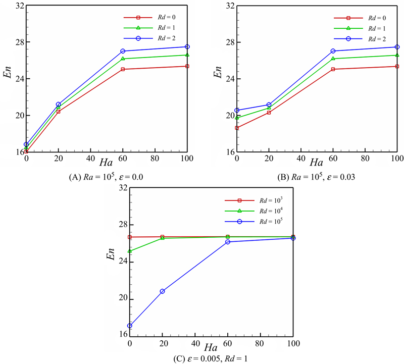
Figure 4.6 Effects of radiation parameter, viscous dissipation parameter, Hartmann number, and Rayleigh number on ratio of enhancement when Pr = 6.2.
4.2. Unsteady nanofluid flow and heat transfer in the presence of magnetic field considering thermal radiation
4.2.1. Problem definition
Heat and mass transfer analysis in the unsteady two-dimensional squeezing nanofluid flow between the infinite parallel plates is considered (Fig. 4.7) [4]. The two plates are placed at  . When γ > 0 the two plates are squeezed until they touch t = 1/γ, and for γ < 0 the two plates are separated. The viscous dissipation effect, the generation of heat due to friction caused by shear in the flow, is retained.

Figure 4.7 Geometry of problem.
The governing equations for momentum, energy, and mass transfer in unsteady two-dimensional flow of nanofluid are as follows:
(4.21)
 (4.22)
 (4.23)
 (4.24)
 (4.25)
where the radiation heat flux qr is considered according to Rosseland approximation such that where σe and βR are the Stefan–Boltzmann constant and the mean absorption coefficient, respectively. The fluid-phase temperature differences within the flow are assumed to be sufficiently small, so that T4 may be expressed as a linear function of temperature. This is done by expanding T4 in a Taylor series about the temperature Tc and neglecting higher order terms to yield, .
where σe and βR are the Stefan–Boltzmann constant and the mean absorption coefficient, respectively. The fluid-phase temperature differences within the flow are assumed to be sufficiently small, so that T4 may be expressed as a linear function of temperature. This is done by expanding T4 in a Taylor series about the temperature Tc and neglecting higher order terms to yield, Here u and  are the velocities in the x- and y-directions, respectively. T is the temperature, C is the concentration, P is the pressure, ρf is the base fluid’s density, μ is the dynamic viscosity, k is the thermal conductivity, cP is the specific heat of nanofluid, DB is the diffusion coefficient of the diffusing species. The relevant boundary conditions are as follows:
 (4.26)
We introduce these parameters:
 (4.27)
Substituting the above variables into (4.22) and (4.23) and then eliminating the pressure gradient from the resulting equations gives:
 (4.29)
 (4.30)
With these boundary conditions:
 (4.31)
where ![]() is the squeeze number, Pr is the Prandtl number, Ec is the Eckert number, Sc is the Schmidt number, Rd is radiation parameter, Nb is the Brownian motion parameter, and Nt is the thermophoretic parameter, which are defined as:
is the squeeze number, Pr is the Prandtl number, Ec is the Eckert number, Sc is the Schmidt number, Rd is radiation parameter, Nb is the Brownian motion parameter, and Nt is the thermophoretic parameter, which are defined as:
 (4.32)
Nusselt number is defined as:
 (4.33)
In terms of (4.27), we obtain
 (4.34)
4.2.2. Effects of active parameters
Unsteady nanofluid flow between parallel plates is investigated considering thermal radiation. Two-phase model is used to simulate nanofluid properties. The basic partial differential equations are reduced to ordinary differential equations which are solved numerically using the fourth-order Runge–Kutta method. The effects of radiation parameter, squeeze number, Schmidt number, Brownian motion parameter, thermophoretic parameter, and Eckert number on heat and mass characteristics are examined.
Fig. 4.8 shows the effect of squeeze number on velocity, temperature, and concentration profiles. The squeeze number has different effects on vertical velocity profile near each plate: f increases with the increase of S when η > 0.5, but the opposite trend is observed when η < 0.5. Thermal boundary layer thickness decreases with the increase of squeeze number, while the opposite trend is observed for concentration boundary layer thickness. Fig. 4.9 shows the effect of Eckert number on temperature and concentration profiles. The presence of viscous dissipation effects significantly increases the temperature, while concentration decreases with the increase of Eckert number.

Figure 4.8 Effect of squeeze number on velocity, temperature, and concentration profiles when Sc = 0.5, Ec = 0.1, Nb = 0.1, Nt = 0.1, Rd = 2, and Pr = 10.
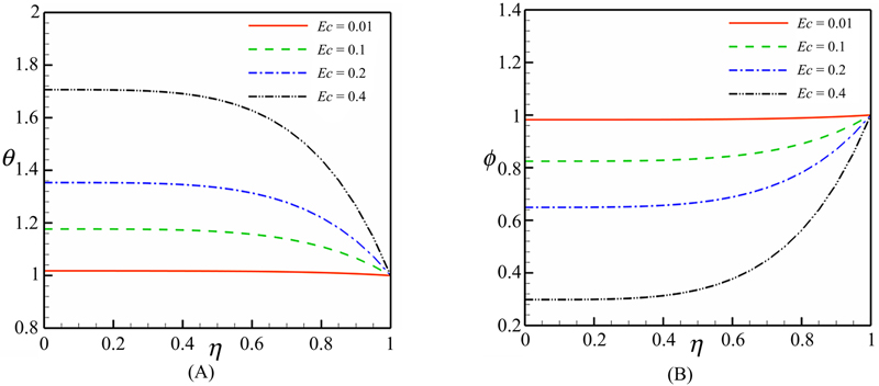
Figure 4.9 Effect of Eckert number on temperature and concentration profiles when S = 0.5, Sc = 0.5, Nb = 0.1, Nt = 0.1, Rd = 2, and Pr = 10.
The effects of thermophoretic parameter and Schmidt number on concentration profile are shown in Fig. 4.10. Increasing thermophoretic parameter causes the concentration to decrease. Schmidt number is a dimensionless number defined as the ratio of momentum diffusivity (viscosity) and mass diffusivity. So, concentration profile increases with the increase of Schmidt number. Fig. 4.11 shows the effect of radiation parameter on temperature and concentration profiles. As radiation parameter increases, temperature boundary layer thickness decreases. Also, this figure shows that concentration increases with the increase of radiation parameter.
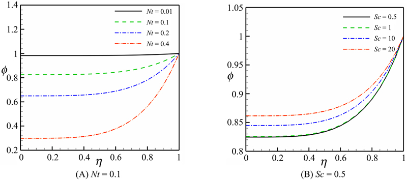
Figure 4.10 Effects of thermophoretic parameter and Schmidt number on concentration profile when S = 0.5, Nb = 0.1, Rb = 2, and Pr = 10.
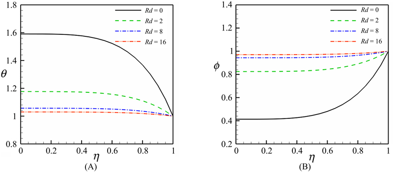
Figure 4.11 Effect of radiation parameter on temperature and concentration profiles when S = 0.5, Sc = 0.5, Ec = 0.1, Nb = 0.1, Nt = 0.1, and Pr = 10.
The effects of Eckert number, Schmidt number, squeeze parameter, and radiation parameter on Nusselt number are shown in Fig. 4.12 and Table 4.1. Nusselt number is an increasing function of Eckert number, Schmidt number, squeeze parameter, and radiation parameter. This observation is due to decreasing boundary layer thickness with the increase of these parameters.

Figure 4.12 Effects of Eckert number, squeeze and radiation parameters on Nusselt number when Sc = 0.5, Nb = 0.1, Nt = 0.2, and Pr = 10.
Table 4.1
Effects of radiation parameter, Schmidt number on Nusselt number when S = 0.5, Ec = 0.01, Nb = 0.1, Nt = 0.2, and Pr = 10
| Sc | ||||
| Rd | 0.5 | 1 | 10 | 20 |
| 0 | 0.27041 | 0.270421 | 0.270507 | 0.270602 |
| 3 | 0.296127 | 0.296127 | 0.29613 | 0.296133 |
| 6 | 0.298606 | 0.298607 | 0.298607 | 0.298608 |
| 12 | 0.299543 | 0.299543 | 0.299543 | 0.299544 |

4.3. Effect of thermal radiation on magnetohydrodynamic nanofluid flow and heat transfer by means of two-phase model
4.3.1. Problem definition
Consider the steady nanofluid flow between two horizontal parallel plates when the fluid and the plates rotate together around the y-axis which is normal to the plates with an angular velocity. A Cartesian coordinate system is considered as follows: the x-axis is along the plate, the y-axis is perpendicular to it, and the z-axis is normal to the x–y plane (Fig. 4.13) [5]. The plates are located at y = 0 and y = h. The lower plate is being stretched by two equal and opposite forces, so that the position of the point (0, 0, 0) remains unchanged. A uniform magnetic flux with density B0 is acting along y-axis about which the system is rotating.
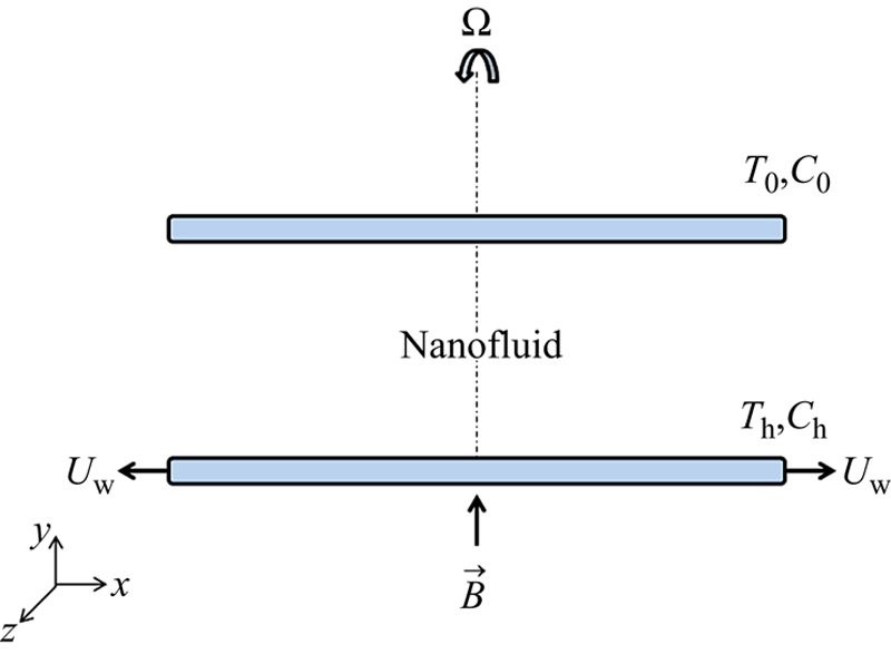
Figure 4.13 Geometry of problem.
The governing equations in a rotating frame of reference are as follows:
 (4.35)
 (4.36)
 (4.37)
 (4.38)
 (4.39)
 (4.40)
where the radiation heat flux qr is considered according to Rosseland approximation such that where σe and βR are the Stefan–Boltzmann constant and the mean absorption coefficient, respectively. The fluid-phase temperature differences within the flow are assumed to be sufficiently small, so that T4 may be expressed as a linear function of temperature [6]. This is done by expanding T4 in a Taylor series about the temperature Tc and neglecting higher order terms to yield, .
where σe and βR are the Stefan–Boltzmann constant and the mean absorption coefficient, respectively. The fluid-phase temperature differences within the flow are assumed to be sufficiently small, so that T4 may be expressed as a linear function of temperature [6]. This is done by expanding T4 in a Taylor series about the temperature Tc and neglecting higher order terms to yield, Here u, , and  are the velocities in the x-, y-, and z-directions, respectively; T is the temperature; C is the concentration; ρf is the base fluid’s density; μ is the dynamic viscosity; k is the thermal conductivity; cP is the specific heat of nanofluid; and DB is the diffusion coefficient of the diffusing species. Also, p* is the modified fluid pressure. The absence of
  in Eq. (4.38) implies that there is a net cross-flow along the z-axis. The relevant boundary conditions are as follows:
in Eq. (4.38) implies that there is a net cross-flow along the z-axis. The relevant boundary conditions are as follows:
 (4.41)
The following nondimensional variables are introduced:
 (4.42)
where a prime denotes differentiation with respect to η.
 (4.43)
 (4.44)
and the nondimensional quantities are defined through in which R is the viscosity parameter, M is the magnetic parameter, and Kr is the rotation parameter.
 (4.46)
Therefore, the governing equations and boundary conditions for this case in nondimensional form are given by:
 (4.51)
 (4.52)
With these boundary conditions:
 (4.53)
where Pr is the Prandtl number, Sc is the Schmidt number, Rd is radiation parameter, Nb is the Brownian motion parameter, and Nt is the thermophoretic parameter, which are defined as:
 (4.54)
Skin friction coefficient Cf along the stretching wall and Nusselt number Nu along the stretching wall are defined as:
 (4.55)
4.3.2. Effects of active parameters
Two-phase simulation of nanofluid flow and heat transfer in the presence of magnetic field is studied considering thermal radiation. To solve numerically the transformed ordinary differential Eqs. (4.49)–(4.52) along with the boundary conditions (4.53), we have used the fourth-order Runge–Kutta method [7].
The effects of Reynolds number, magnetic parameter, rotation parameter, Schmidt number, thermophoretic parameter, Brownian parameter, and radiation parameter on heat and mass characteristics are examined. Fig. 4.14 shows the effects of Reynolds number, magnetic parameter, and rotation parameter on velocity profiles. Reynolds number shows the relative significance of the inertia effect compared with the viscous effect. Thus, velocity boundary layer thickness decreases with the increase of Reynolds number. By increasing the magnetic parameter velocity in y-direction decreases, while the velocity in z-direction increases. This phenomenon is due to the point that variation of magnetic parameter leads to the difference of the Lorentz force due to magnetic field, and the Lorentz force produces more resistance to transport phenomena. The effect of rotation parameter on f(η) is similar to that of magnetic parameter. The Carioles force has inverse effect on g(η) in comparison with Lorenz force, which means that with increasing rotation parameter, the transverse velocity increases.

Figure 4.14 Effects of Reynolds number, magnetic parameter, and rotation parameter on velocity profiles (f, g).
The effects of Reynolds number and radiation parameter on temperature profile are shown in Fig. 4.15. As Reynolds number increases, temperature profile decreases between two plates, while the opposite trend is observed for radiation parameter. Fig. 4.16 depicts the effects of radiation parameter, Reynolds number, thermophoretic parameter, Brownian parameter, and Schmidt number on concentration profile. Concentration profile at middle point increases, as Reynolds number and thermophoretic parameter increase, while it decreases with the increase of radiation parameter, Brownian parameter, and Schmidt number. The effects of active parameters on Nusselt number are shown in Fig. 4.17 and Tables 4.2–4.4. Thermal boundary layer thickness decreases with the increase of radiation parameter and Reynolds number. So, Nusselt number increases with the increase of these parameters. Also, it can be concluded that Nusselt number is a decreasing function of Schmidt number, rotation, Brownian, thermophoretic, and magnetic parameters.
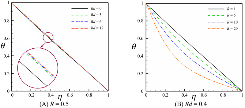
Figure 4.15 Effects of Reynolds number and radiation parameter on temperature profile when Kr = 2, Sc = 0.5, Nt = 0.2, Nb = 0.2, M = 4, and Pr = 10.

Figure 4.16 Effects of radiation parameter, Reynolds number, thermophoretic parameter, Brownian parameter, and Schmidt number on concentration profile when Kr = 2, M = 4, and Pr = 10.
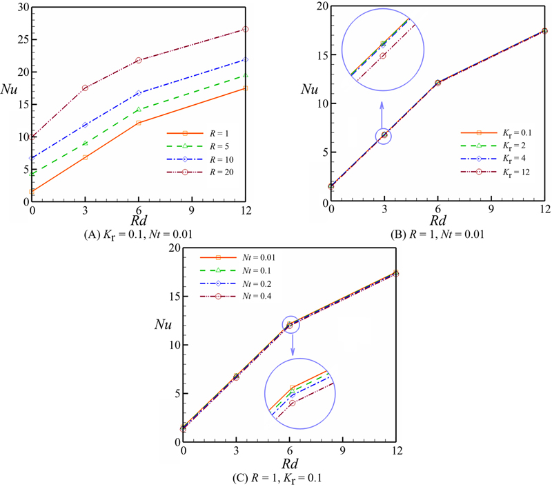
Figure 4.17 Effects of radiation parameter, Reynolds number, rotation parameter, and thermophoretic parameter on Nusselt number when Sc = 0.5, Nb = 0.01, M = 0, and Pr = 10.
Table 4.2
Effects of radiation parameter and Magnetic parameter on Nusselt number when Sc = 0.5, Nb = 0.01, R = 1, Kr = 0.1, Nt = 0.01, and Pr = 10
| M | ||||
| Rd | 0 | 4 | 8 | 16 |
| 0 | 1.557044 | 1.523667 | 1.4954 | 1.449936 |
| 3 | 6.830242 | 6.802148 | 6.778303 | 6.739817 |
| 6 | 12.1581 | 12.13053 | 12.10713 | 12.06931 |
| 12 | 17.48938 | 17.46202 | 17.43877 | 17.40121 |

Table 4.3
Effects of radiation parameter and Schmidt number on Nusselt number when Nb = 0.01, M = 0, R = 1, Kr = 0.1, Nt = 0.01, and Pr = 10
| Sc | ||||
| Rd | 0.01 | 0.2 | 2 | 6 |
| 0 | 1.557044 | 1.557021 | 1.556798 | 1.556285 |
| 3 | 6.830242 | 6.830225 | 6.830065 | 6.829702 |
| 6 | 12.1581 | 12.15808 | 12.15792 | 12.15757 |
| 12 | 17.48938 | 17.48936 | 17.48921 | 17.48886 |

Table 4.4
Effects of radiation parameter and Brownian parameter on Nusselt number when Sc = 0.5, M = 0, R = 1, Kr = 0.1, Nt = 0.01, and Pr = 10
| Nb | ||||
| Rd | 0.01 | 0.1 | 0.3 | 0.6 |
| 0 | 1.557044 | 1.49911 | 1.37463 | 1.199351 |
| 3 | 6.830242 | 6.783053 | 6.678947 | 6.524752 |
| 6 | 12.1581 | 12.1119 | 12.00966 | 11.85736 |
| 12 | 17.48938 | 17.44356 | 17.34201 | 17.19043 |

..................Content has been hidden....................
You can't read the all page of ebook, please click here login for view all page.