
6.7. Simulation of MHD CuO–water nanofluid flow and convective heat transfer considering Lorentz forces
6.7.1. Problem definition
The numerical model consists in a two-dimensional square cavity with side equal to H which represents the characteristic dimension of the problem (Fig. 6.39A) [14]. The heat source is centrally located on the bottom surface and its length 1 varied from 2/5 to 4/5 of H; the ratio 1/H is called ɛ. The cooling is achieved by the two vertical walls. The heat source has a temperature Th, while the cooling walls have a temperature Tc; all the other surfaces are adiabatic (Th > Tc). Also, it is also assumed that the uniform magnetic field ( ) of constant magnitude
  is applied, where
  and
and  are unit vectors in the Cartesian coordinate system. The orientation of the magnetic field forms an angle θM with horizontal axis such that θM = cot−1(Bx/By). The electric current J and the electromagnetic force F are defined by
  and
and  , respectively. The governing equations are similar to those of exist in Section 6.1.1. To compare total heat transfer rate, Nusselt number is used. The local and average Nusselt numbers on cold enclosure are defined as follows:
) of constant magnitude is applied, where 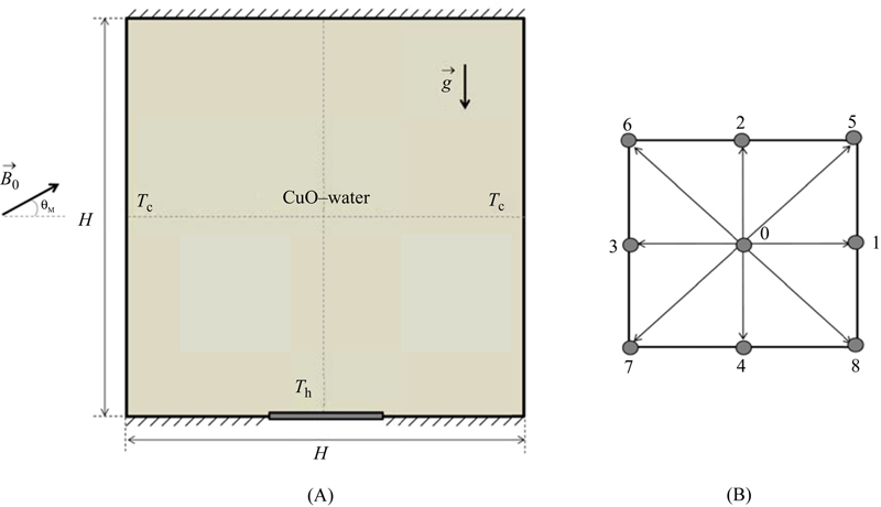
Figure 6.39 (A) Geometry of the problem; (B) discrete velocity set of two-dimensional nine-velocity (D2Q9) model.
 (6.101)
6.7.2. Effects of active parameters
Effect of horizontal magnetic field on development of the heat transfer phenomenon in a square enclosure partially heated from below is investigated. LBM scheme was utilized to obtain the numerical simulation in a cavity filled with CuO–water. The present numerical solution is validated by comparing the present code results against the results of Calcagni et al. [15] for viscous flow (φ = 0) (Fig. 6.40). Effect of active parameters such as Rayleigh number (Ra = 103, 104, and 105), Hartmann number (Ha = 0, 20, 60, and 100), heat source length (ɛ = 1/H = 0.4, 0.6, and 0.8), and volume fraction of nanoparticle (φ = 0 and 0.04) on flow and heat transfer are examined.

Figure 6.40 Comparison of isotherms between the present work and experimental and numerical study of Calcagni et al. [15].
Fig. 6.41 depicts the effect of volume fraction of nanoparticle on streamlines and isotherms. As seen the velocity components increase with the increase of nanoparticles volume fraction which enhances the energy transport within the fluid. Thus, the absolute values of stream functions indicate that the strength of flow increases with the increase of the volume fraction of nanoparticle. The sensitivity of thermal boundary layer thickness to volume fraction of nanoparticles is related to the increased thermal conductivity of the nanofluid. In fact, higher values of thermal conductivity are accompanied by higher values of thermal diffusivity. The high value of thermal diffusivity causes a drop in the temperature gradients and accordingly increases the boundary layer thickness. Although adding nanoparticles leads to increase thermal boundary layer thickness, Nusselt number increases because it is a multiplication of temperature gradient and the thermal conductivity ratio. Reduction in temperature gradient is much smaller than the thermal conductivity ratio.
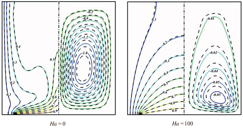
Figure 6.41 Comparison of the isotherms (left) and streamlines (right) contours between nanofluid (φ = 0.04) (- - -) and pure fluid (φ = 0) (––) when ɛ = 0.8, Ra = 105.
Effects of Rayleigh number, heat source length, and Hartmann number on isotherms (left) and streamlines (right) contours are shown in Figs. 6.42–6.44. By increasing Rayleigh number, the buoyancy forces increase and overcome the viscous forces, and the heat transfer is dominated by convection at high Rayleigh number. Moreover, the isotherms are more distorted at higher Rayleigh numbers due to the stronger convection effects. Increasing Hartmann number causes Lorenz force to increase and leads to a substantial suppression of the convection. The core of main cell moves downward with the increase of Hartmann number. As Lorentz forces increase, the conduction heat transfer mechanism is more marked and isotherms are parallel to each other. Also, it can be seen that the absolute values of stream function increase with the increase of heat source length. Thermal boundary layer thickness near the bottom wall decreases with the augment of ɛ. Effects of heat source length and Hartmann number on flow and heat transfer are more sensible for high Rayleigh number.

Figure 6.42 Effects of heat source length and Hartmann number on isotherms (left) and streamlines (right) contours when φ = 0.04, Ra = 103.
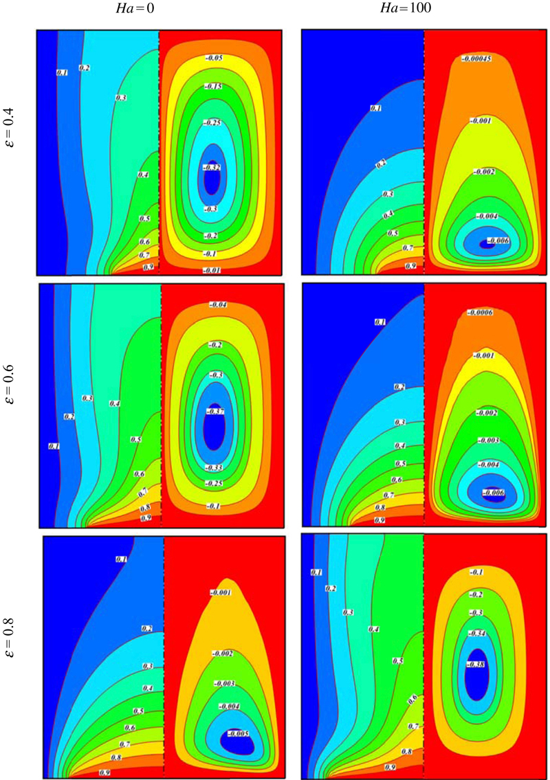
Figure 6.43 Effects of heat source length and Hartmann number on isotherms (left) and streamlines (right) contours when φ = 0.04, Ra = 104.

Figure 6.44 Effects of heat source length and Hartmann number on isotherms (left) and streamlines (right) contours when φ = 0.04, Ra = 105.
Fig. 6.45 shows the effects of Rayleigh number, Hartmann number, and heat source length on average Nusselt number. Nusselt number increases with the increase of Rayleigh number and heat source length, while it decreases with the increase of Hartmann number. Effects of Rayleigh number, heat source length, and Hartmann number on heat transfer enhancement are depicted in Fig. 6.46. It can be found that the effect of nanoparticles is more obvious at low Rayleigh number than at high Rayleigh number. This observation can be clarified by noting that at low Rayleigh number the heat transfer is dominant by conduction. Therefore, the addition of high thermal conductivity nanoparticles will increase the conduction and so make the enhancement more effective. Also, this figure depicts that increasing Hartmann number leads to increase in heat transfer enhancement. Furthermore, rate of enhancement increases with the increase of heat source length.

Figure 6.45 Effects of Rayleigh number, heat source length, and Hartmann number on average Nusselt number when φ = 0.04.

Figure 6.46 Effects of Rayleigh number, heat source length, and Hartmann number on heat transfer enhancement.
6.8. Three-dimensional mesoscopic simulation of magnetic field effect on natural convection of nanofluid
6.8.1. Problem definition
The numerical model consists in a three-dimensional square cavity with side equal to L which represents the characteristic dimension of the problem (Fig. 6.47) [16]. The hot and cold wall were located at Z = z/L = 0 and Z = z/L = 1, respectively. All the other surfaces are adiabatic. Also, it is also assumed that the uniform magnetic field ( ) of constant magnitude
  is applied, where , , and
  are unit vectors in the Cartesian coordinate system. The orientation of the magnetic field forms an angle θz with z axis and θx with x axis. The electric current J and the electromagnetic force F are defined by and , respectively. In this chapter, θx = θz = 90°.
is applied, where 
Figure 6.47 Geometry of the problem.
The thermal LB model utilizes two distribution functions, f and g, for the flow and temperature fields, respectively. It uses modeling of movement of fluid particles to capture macroscopic fluid quantities such as velocity, pressure, and temperature. In this approach, the fluid domain discretized to uniform Cartesian cells. Each cell holds a fixed number of distribution functions, which represent the number of fluid particles moving in these discrete directions. The density and distribution functions, that is, the f and g, are calculated by solving the lattice Boltzmann equation, which is a special discretization of the kinetic Boltzmann equation. After introducing BGK approximation, the general form of lattice Boltzmann equation with external force is as follows.
For the flow field:
 (6.102)
For the temperature field:
 (6.103)
where ∆t denotes lattice time step, ci is the discrete lattice velocity in direction i, Fk is the external force in direction of lattice velocity, and τv and τc denote the lattice relaxation time for the flow and temperature fields. The kinetic viscosity υ and the thermal diffusivity α are defined in terms of their respective relaxation times, that is,  and
and  , respectively. Note that the limitation 0.5 < τ should be satisfied for both relaxation times to ensure that viscosity and thermal diffusivity are positive. Furthermore, the local equilibrium distribution function determines the type of problem that needs to be solved. The D3Q19 model was used (Fig. 6.48). These 19 velocities are given as follows [17].
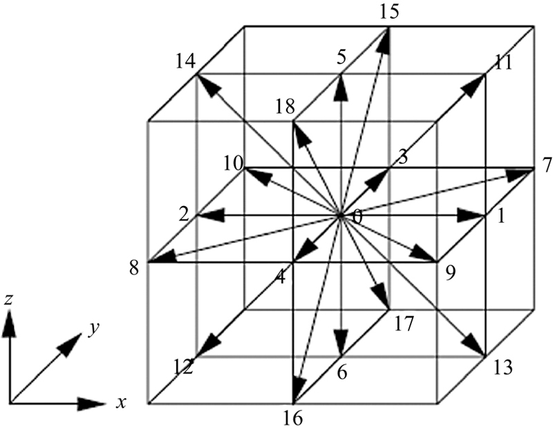
Figure 6.48 Discrete velocity for the D3Q19 model.
 (6.104)
It also models the equilibrium distribution functions, which are calculated with Eqs. (6.105) and (6.106) for flow and temperature fields, respectively.
 (6.105)
 (6.106)
where ρ and T are the lattice fluid density and temperature.
Weighting factor (wi) is defined as follows:
 (6.107)
To incorporate buoyancy forces and magnetic forces in the model, the force term in the Eq. (6.102) needs to calculate as follows [16]:
 (6.108)
where A is  and
and  is the Hartmann number.
and is the Hartmann number.For natural convection, the Boussinesq approximation is applied and radiation heat transfer is negligible. To ensure that the code works in near incompressible regime, the characteristic velocity of the flow for natural  regime must be small compared with the fluid speed of sound. In this chapter, the characteristic velocity selected as 0.1 of sound speed.
Finally, macroscopic variables calculate with the following formula:
 (6.109)
To simulate the nanofluid by the LBM, because of the interparticle potentials and other forces on the nanoparticles, the nanofluid behaves differently from the pure liquid from the mesoscopic point of view and is of higher efficiency in energy transport as well as better stabilization than the common solid–liquid mixture. For modeling the nanofluid because of changing in the fluid thermal conductivity, density, heat capacitance, and thermal expansion, some of the governed equations should change. The effective density (ρnf), the effective heat capacity (ρCp)nf, thermal expansion (ρβ)nf, and electrical conductivity (σ)nf of the nanofluid are defined as
 (6.113)
where φ is the solid volume fraction of the nanoparticles and subscripts f, nf, and s stand for base fluid, nanofluid, and solid, respectively.
 (6.114)
 (6.115)
To compare total heat transfer rate, Nusselt number is used. The local and average Nusselt numbers on hot wall are defined as follows:
 (6.116)
To estimate the enhancement of heat transfer between the case of φ = 0.04 and the pure fluid (base fluid) case, the heat transfer enhancement is defined as
 (6.117)
The kinetic energy of the fluid is defined as follows:
6.8.2. Effects of active parameters
A numerical investigation is presented for free convection heat transfer of Al2O3–water nanofluid in the presence of magnetic field parallel to gravity in a cubic cavity heated from below. The governing equations are solved via LBM. Computations are carried out for different values of Rayleigh number (Ra = 103, 104, and 105), Hartmann number (Ha = 0, 20, 40, and 60), and volume fraction of nanoparticle (φ = 0 and 0.04).
Effects of Hartmann number and Rayleigh number on isotherm, streamlines, and isokinetic energy are shown in Figs. 6.49–6.51. All the contours are symmetric with respect to the vertical midplane of the enclosure due to symmetrical boundary conditions. In general, natural convection of nanofluid in the enclosure is affected by buoyancy and Lorentz forces. The buoyancy force has an aiding effect on natural convection, but the Lorentz force has an opposing effect. Either of the two forces is important, when Ha2/Ra ≈ 1. The buoyancy force is dominant when Ha2/Ra ≪ 1 and the Lorentz force is dominant when Ha2/Ra ≫ 1.

Figure 6.49 Effect of Hartmann number on (A) isotherm, (B) streamlines, and (C) isokinetic energy at Y = y/L = 0.5 when Ra = 103, φ = 0.04.

Figure 6.50 Effect of Hartmann number on (A) isotherm, (B) streamlines, and (C) isokinetic energy at Y = y/L = 0.5 when Ra = 104, φ = 0.04.
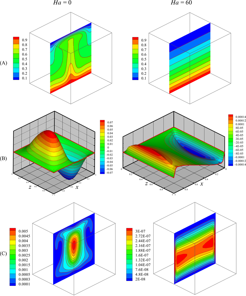
Figure 6.51 Effect of Hartmann number on (A) isotherm, (B) streamlines, and (C) isokinetic energy at Y = y/L = 0.5 when Ra = 105, φ = 0.04.
At low Rayleigh number, conduction is the main heat transfer mechanism number. So, the shape of the isotherms tends to follow the geometry of the enclosure. The maximum value of stream function can be viewed as a measure of the intensity of natural convection in the cavity. It is evident from the figures that by increasing the Ra, the maximum value of the stream function increases; this means that the flow moves faster as natural convection is stronger and the isotherm will be distorted. For high Rayleigh number, where buoyancy forces are more dominant than the viscous forces, the convection currents inside the enclosure become very strong. As the cold fluid has a downward motion with an increase of circular flow, the convection becomes the basic mode of heat transfer. By increasing all Rayleigh numbers, the Hartmann numbers have a pure conduction regime because Lorentz force interacts with the buoyancy force and suppresses the convection flow by reducing the velocities. Furthermore, it is shown that as the Rayleigh number is increased, the convective heat transfer is also increased so that for suppression of convection higher magnetic field is needed. By increasing magnetic field, the alteration in the temperature distribution seems to be more serious. The thermal boundary layers at the two isothermal walls die out, indicating the weakened role of the convection in the heat transfer mechanism. Also, it can be found that the maximum value of stream function decreases with the increase of Hartmann number. At Ra = 103, contour of kinetic energy shows a single cell. Lorentz forces elongated this cell along the horizontal axis. As Rayleigh number increases up to 104, two smaller cells appear near the vertical wall. At Ra = 105, the main cell of isokinetic energy is elongated along the vertical axis. Also, it can be found that kinetic energy increases with the increase of Rayleigh number, but it decreases with the augment of Hartmann number.
Effects of Rayleigh number and Hartmann number on local and average Nusselt number on hot wall are depicted in Figs. 6.52 and 6.53A. Thermal boundary layer thickness increases with the augment of Hartmann number, while it decreases with the increase of Rayleigh number. So, Nusselt number has direct relationship with Rayleigh number, but it has inverse relationship with Hartmann number. Fig. 6.53B shows the effects of Rayleigh number and Hartmann number on heat transfer enhancement. It is noteworthy that the heat transfer enhancement becomes its maximum value at low Raleigh number and high Hartmann number. This observation is due to domination of conduction in this case. So, the addition of high thermal conductivity nanoparticles will increase the conduction and therefore make the enhancement more effective.

Figure 6.52 Effects of Rayleigh number and Hartmann number on local Nusselt number on hot wall when φ = 0.04.
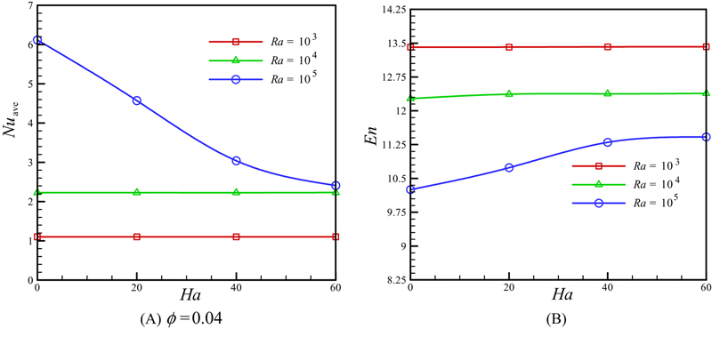
Figure 6.53 Effects of Rayleigh number and Hartmann number on average Nusselt and heat transfer enhancement.
6.9. Two-phase simulation of nanofluid flow and heat transfer in an annulus in the presence of an axial magnetic field
6.9.1. Problem definition
Flow is assumed to be steady, laminar, and unidirectional; therefore, the radial and axial components of the velocity and the derivatives of the velocity with respect to θ and z are zero (Fig. 6.54) [18]. Under these assumptions and in cylindrical coordinates, the governing equations for nanofluid flow, heat, and mass transfer following the azimuthal direction can be defined as follows:
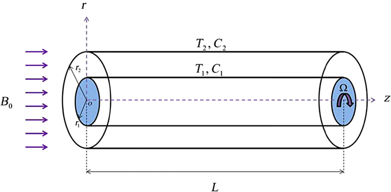
Figure 6.54 Geometry of the problem.
 (6.119)
 (6.120)
 (6.121)
 (6.122)
The governing equation and boundary conditions, Eqs. (6.119)–(6.122), which are in nondimensional form, become
 (6.123)
 (6.124)
 (6.125)
 (6.126)
where
 (6.127)
Nusselt number Nu along the inner wall is defined as
 (6.128)
6.9.2. Effects of active parameters
Flow, heat, and mass transfer of Al2O3–water nanofluid between two horizontal coaxial cylinders in the presence of an axial magnetic field are investigated. Two-phase model is used for simulation of nanofluid flow and heat transfer. ODEs along with initial conditions are solved using the fourth-order Runge–Kutta integration technique [19]. The effects of Hartmann number, Reynolds number, Schmidt number, Brownian parameter, thermophoresis parameter, Eckert number, and aspect ratio on flow, heat, and mass transfer characteristics are examined.
Effects of Hartmann number and Reynolds number on velocity, temperature, and concentration profiles are shown in Figs. 6.55 and 6.56. Hartmann number is the ratio of electromagnetic force to the viscous force. Lorentz forces increase with the increase of Hartmann number and in turn the velocity decreases with the increase of Hartmann number. As Hartmann number increases temperature profiles decrease, but the concentration profile increases. Reynolds number is the ratio of inertial forces to viscous forces. Increasing Reynolds number leads to increase in velocity and temperature profiles, but opposite trend is observed for concentration profile.
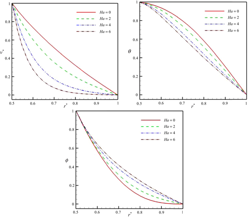
Figure 6.55 Effect of Hartmann number on velocity, temperature, and concentration profiles when Pr = 10, η = 0.5, Ec = 0.01, Re = 1, Sc = 1, Nb = 0.1, Nt = 0.1.

Figure 6.56 Effect of Reynolds number on velocity, temperature, and concentration profiles when Pr = 10, η = 0.5, Ha = 1, Ec = 0.01, Sc = 1, Nb = 0.1, Nt = 0.1.
Fig. 6.57 shows the effects of Hartmann number and Reynolds number on Nusselt number. Increasing the Hartmann number leads to increase in temperature boundary layer thickness, while the opposite trend is observed for the Reynolds number. So, Nusselt number increases with increasing Hartmann number, while it decreases with increasing Reynolds number.
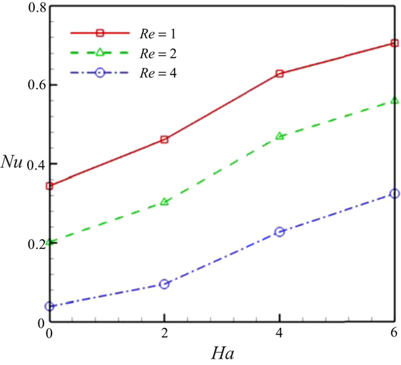
Figure 6.57 Effect of Reynolds number and Hartmann number on Nusselt number when Pr = 10, η = 0.5, Ec = 0.01, Sc = 1, Nb = 0.1, Nt = 0.1.
Fig. 6.58 depicts the effect of the Brownian parameter on temperature, concentration profiles, and Nusselt number. By increasing Brownian motion parameter, thermal diffusivity decreases and in turn thermal boundary layer thickness increases. So, rate of heat transfer decreases with the increase of Brownian motion parameter. Also, it can be found that concentration boundary layer increases with the increase of Brownian motion parameter. Fig. 6.59 depicts the effect of the thermophoresis parameter on the concentration profiles and Nusselt number. Effect of the thermophoresis parameter on the Nusselt number is similar to that of the Brownian parameter. Increasing the thermophoresis parameter leads to increase in the concentration boundary layer. The Nusselt number decreases as the thermophoresis parameter increases.
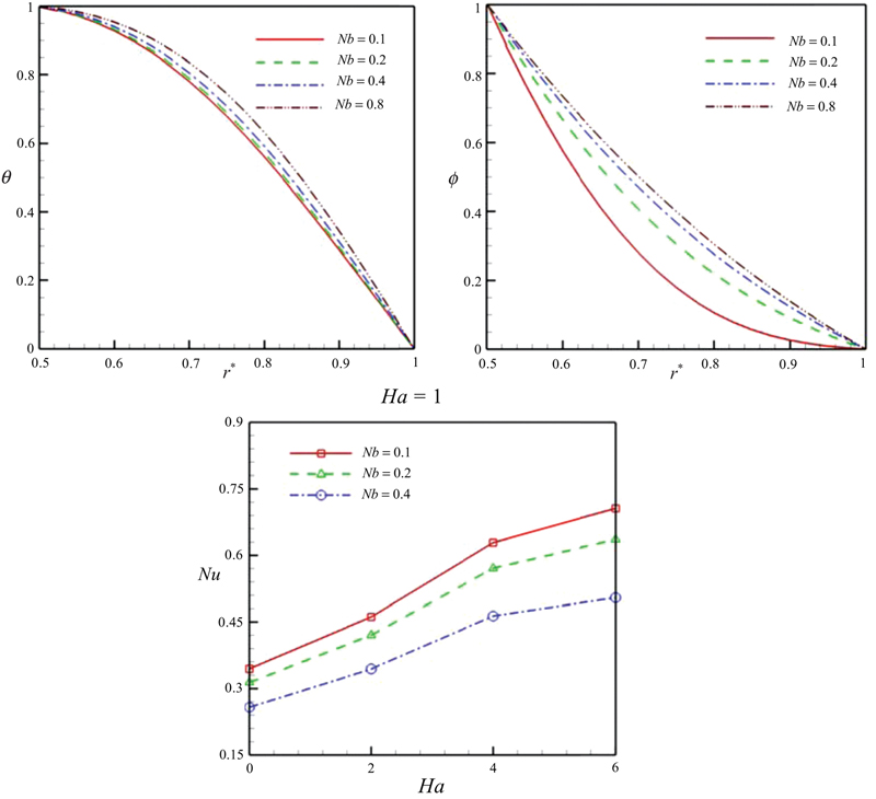
Figure 6.58 Effect of Brownian parameter on temperature, concentration profiles, and Nusselt number when Pr = 10, η = 0.5, Ec = 0.01, Re = 1, Sc = 1, Nt = 0.1.
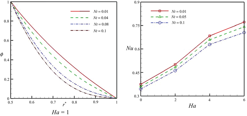
Figure 6.59 Effect of thermophoresis parameter on concentration profile and Nusselt number when Pr = 10, η = 0.5, Ec = 0.01, Re = 1, Sc = 1, Nb = 0.1.
Fig. 6.60 shows the effect of the Eckert number on the temperature profile and Nusselt number. As the Eckert number increases, viscous dissipation increases and in turn the temperature increases and Nusselt number decreases. Effect of the Schmidt number on the concentration profile is depicted in Fig. 6.61 and Table 6.6. Concentration increases with the increase of Schmidt number, while the thermal boundary layer thickness decreases. So, Nusselt number increases with the increase of Schmidt number. Fig. 6.62 shows the effect of the aspect ratio on the Nusselt number. As the aspect ratio increases, the distance between the hot and cold walls of the horizontal coaxial cylinders decreases and the Nusselt number increases.
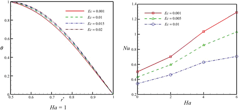
Figure 6.60 Effect of Eckert number on temperature profile and Nusselt number when Pr = 10, η = 0.5, Re = 1, Sc = 1, Nb = 0.1, Nt = 0.1.

Figure 6.61 Effect of Schmidt number on concentration profile when Pr = 10, η = 05, Ha = 1, Ec = 0.01, Re = 1, Nb = 0.1, Nt = 0.1.
Table 6.6
Effect of Schmidt number on concentration when Pr = 10, η = 0.5, Ec = 0.01. Re = 1, Nb = 0.1, Nt = 0.1
| Ha | Sc | ||
| 0.5 | 1 | 2 | |
| 0 | 0.343909 | 0.344245 | 0.344933 |
| 2 | 0.461028 | 0.461393 | 0.46213 |
| 4 | 0.628474 | 0.628794 | 0.629434 |
| 6 | 0.705387 | 0.705624 | 0.706094 |


Figure 6.62 Effect of aspect ratio on Nusselt number when Pr = 10, Ec = 0.01, Re = 1, Sc = 1, Nb = 0.1, Nt = 0.1.
The corresponding polynomial representation of such model for Nusselt number is as follows:
 (6.129)
Table 6.7
Constant coefficient for using Eq. (6.129)
| aij | i = 1 | i = 2 | i = 3 | i = 4 | i = 5 | i = 6 |
| j = 1 | 0.306009 | 1.185703 | −2.24994 | −0.38755 | 6.581819 | −2.16197 |
| j = 2 | 4.757492 | −6.27872 | −1.12292 | 2.132729 | 46.88285 | −2.22654 |
| j = 2 | 2.756484 | −11.9752 | 0.124053 | 14.13088 | −0.00312 | −0.07635 |
| j = 3 | −0.37891 | −0.55728 | 0.378953 | 1.631652 | 0.788778 | 0.06663 |
| j = 4 | −0.16013 | 34.84572 | 2.02581 | −1219.24 | 0.107653 | −128.364 |
| j = 5 | −0.69095 | 2.318391 | 1.015165 | −1.70229 | 0.019379 | −0.10102 |
| j = 6 | 0.306009 | 1.185703 | −2.24994 | −0.38755 | 6.581819 | −2.16197 |

6.10. Magnetic field effect on unsteady nanofluid flow and heat transfer using Buongiorno model
6.10.1. Problem definition and semianalytical method
6.10.1.1. Problem statement
Heat and mass transfer analysis in the unsteady two-dimensional squeezing flow of nanofluid between the infinite parallel plates is considered (Fig. 6.63) [20]. The two plates are placed at  . When β > 0 the two plates are squeezed until they touch t = 1/β and for β < 0 the two plates are separated. The viscous dissipation effect, the generation of heat due to friction caused by shear in the flow, is retained. Also, it is also assumed that the uniform magnetic field (
 ) is applied, where is unit vectors in the Cartesian coordinate system. The electric current J and the electromagnetic force F are defined by and , respectively.
) is applied, where 
Figure 6.63 Geometry of problem.
The governing equations for mass, momentum, energy, and mass transfer in unsteady two-dimensional flow of nanofluid are as follows:
 (6.130)
 (6.131)
 (6.132)
 (6.133)
 (6.134)
where the radiation heat flux qr is considered according to Rosseland approximation such that  where σe and βR are the Stefan–Boltzmann constant and the mean absorption coefficient, respectively. The fluid-phase temperature differences within the flow are assumed to be sufficiently small, so that T4 may be expressed as a linear function of temperature. This is done by expanding T4 in a Taylor series about the temperature Tc and neglecting higher order terms to yield
  .
.
where σe and βR are the Stefan–Boltzmann constant and the mean absorption coefficient, respectively. The fluid-phase temperature differences within the flow are assumed to be sufficiently small, so that T4 may be expressed as a linear function of temperature. This is done by expanding T4 in a Taylor series about the temperature Tc and neglecting higher order terms to yield Here u and v are the velocities in the x and y directions, respectively; T is the temperature; C is the concentration; P is the pressure; ρf is the base fluid’s density; μ is the dynamic viscosity; k is the thermal conductivity; cP is the specific heat of nanofluid; and DB is the diffusion coefficient of the diffusing species. The relevant boundary conditions are as follows:
 (6.135)
We introduce these parameters:
 (6.136)
Substituting the above variables into (6.131) and (6.132) and then eliminating the pressure gradient from the resulting equations gives:
 (6.138)
 (6.139)
With these boundary conditions:
 (6.140)
where S is the squeeze number, Pr is the Prandtl number, Ec is the Eckert number, Sc is the Schmidt number, Ha is Hartman number of nanofluid, Nb is the Brownian motion parameter, Nt is the thermophoretic parameter, and Rd is the Radiation parameter, which are defined as
 (6.141)
Skin friction coefficient and Nusselt number are defined as
6.10.1.2. DTM solution
 (6.144)
 (6.146)
 (6.148)
By solving the above equations:
 (6.150)
 (6.151)
 (6.152)
Finally we have:
 (6.153)
 (6.155)
6.10.2. Effects of active parameters
Unsteady nanofluid flow and heat transfer between parallel sheets is studied considering Buongiorno model using DTM. The influences of the squeeze number, radiation parameter, Hartmann number, Brownian motion parameter, thermophoretic parameter, and Eckert number on heat and mass characteristics are examined.
Effects of the Hartmann and squeeze numbers on the velocity profiles and skin friction coefficient are demonstrated in Fig. 6.64. It is significant to reminder that the squeeze number (S) defines the movement of the sheets (S > 0 corresponds to the plates moving apart, while S < 0 corresponds to the plates moving together). In this chapter, positive values of squeeze number are examined. Squeeze number has different effects on vertical velocity profile near each sheet: f′ increases with the increase of S when η > 0.5, but opposite trend is detected when η < 0.5. It is valuable saying that the impact of magnetic field is to reduce the value of the velocity magnitude near the lower plat because the existence of magnetic field presents a force called the Lorentz force, which acts in contradiction of the flow. This type of resisting force slows down the fluid velocity. Also, it can be concluded that skin friction coefficient augments with the enhancement of Hartmann number and squeeze number.
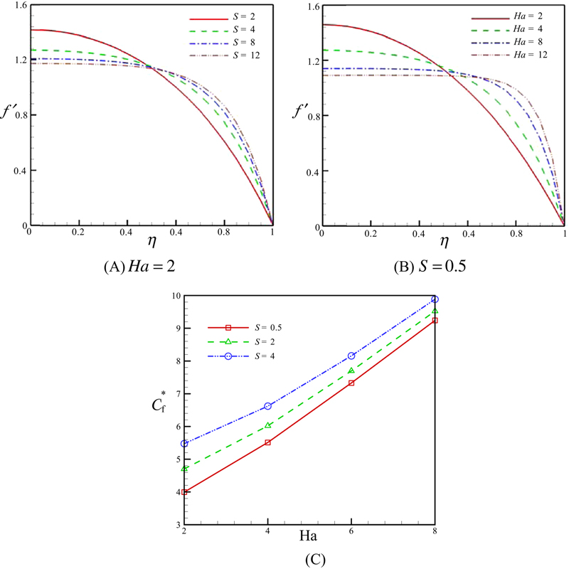
Figure 6.64 Effects of the squeeze number and Hartmann number on the velocity profile and skin friction coefficient.
Fig. 6.65 shows the effect of the radiation parameter, squeeze number, Hartmann number and Nt on the temperature profile. Effects of active parameters on Nusselt number are depicted in Figs. 6.66 and 6.67. The corresponding polynomial representation for Nusselt number is as follows:

Figure 6.65 Effects of the radiation parameter, squeeze number, Hartmann number, and Nt on the temperature profile when Sc = 0.5, Nb = 0.1, Ec = 0.1, and Pr = 10.
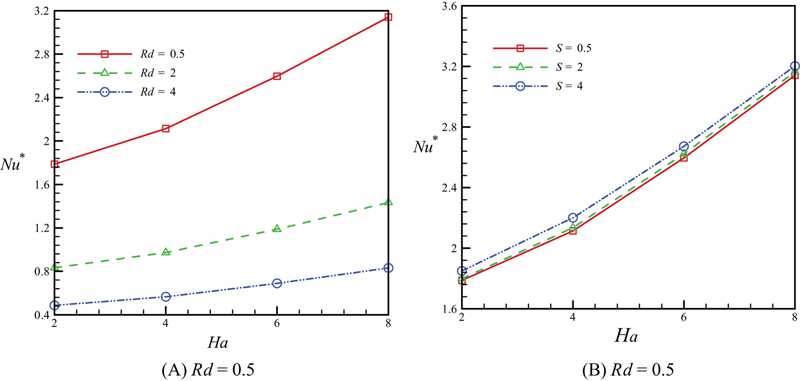
Figure 6.66 Effects of the radiation parameter, squeeze number, and Hartmann number on Nusselt number when Sc = 0.5, Nb = 0.1, Ec = 0.1, Nt = 0.1, and Pr = 10.
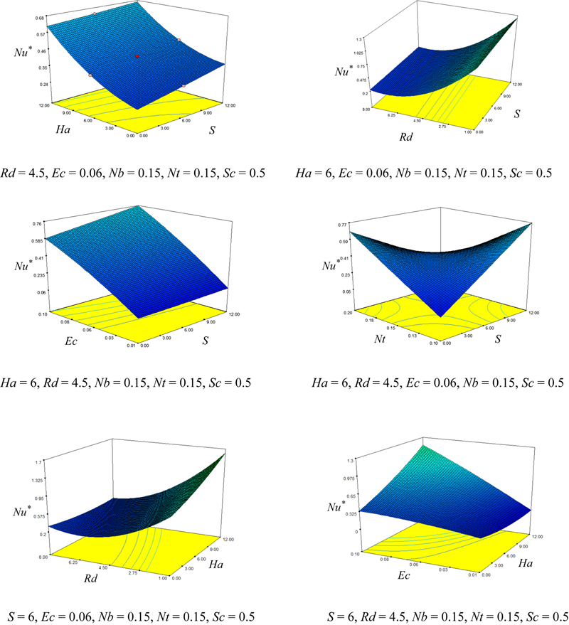
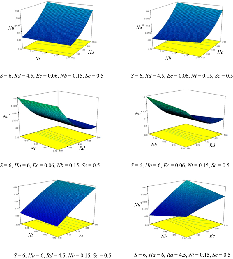
Figure 6.67 Effect of active parameters on Nusselt number.
 (6.156)
As radiation parameter augments, thermal boundary layer thickness near the upper wall augments. So, Nusselt number reduces with the augment of this parameter. The enhancement in the squeeze number can be associated with reducing in the kinematic viscosity, an augment in the distance between the plates and an augment in the speed at which the plates move. Thermal boundary layer thickness near the upper wall reduces as the squeeze number augments. Temperature profiles have meeting point near η = 0.82 for different values of Hartmann number. Increasing Hartmann number leads to augment in temperature profile gradient near the hot plate. Nusselt number enhances with the rise of Hartmann number and squeeze number. Nusselt number augments slightly as Nt increases due to decrease in thermal boundary thickness near the upper plate.
Effects of the radiation parameter, squeeze number, Hartmann number, Nt, and Nb on the concentration profile are shown in Fig. 6.68. Concentration profile enhances with the augment of squeeze number, radiation parameter, and Nb, but it reduces with the increase of Nt. As Hartmann number increases, concentration enhances when η < 0.82, but opposite trends observed when η > 0.82.
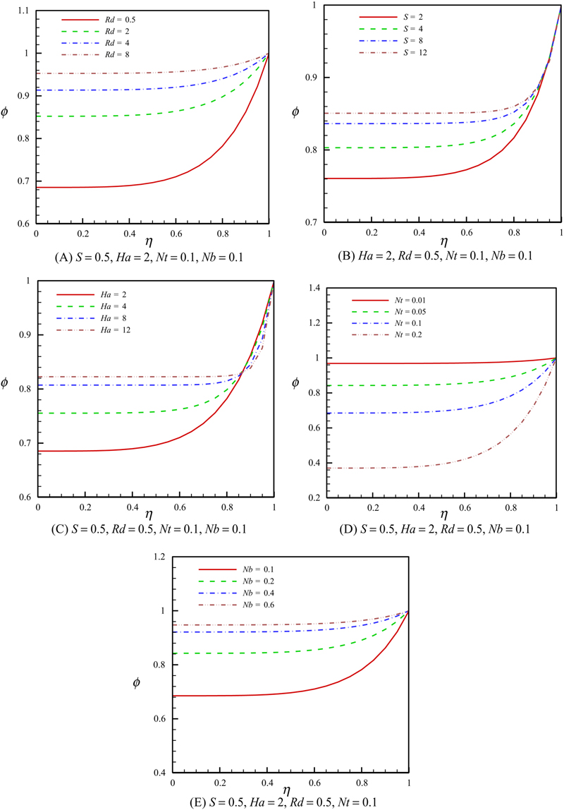
Figure 6.68 Effects of the radiation parameter, squeeze number, Hartmann number Nt and Nb on the concentration profile when Sc = 0.5, Ec = 0.1, and Pr = 10.
6.11. Free convection of magnetic nanofluid considering MFD viscosity effect
6.11.1. Problem definition
The geometry of this section is shown in Fig. 6.69A [21]. The heat source is centrally located on the bottom surface and its length L/3. The cooling is achieved by the two vertical walls. The heat source has constant heat flux q″, while the cooling walls have a constant temperature Tc; all the other surfaces are adiabatic. Also, it is also assumed that the uniform magnetic field () of constant magnitude is applied, where and are unit vectors in the Cartesian coordinate system. The orientation of the magnetic field forms an angle θM with horizontal axis such that θM = cot−1(Bx/By). The electric current J and the electromagnetic force F are defined by and , respectively.
) of constant magnitude is applied, where 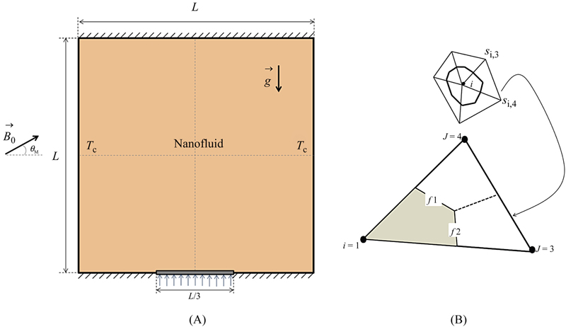
Figure 6.69 (A) Geometry and the boundary conditions; (B) a sample triangular element and its corresponding control volume.
The flow is steady, two-dimensional, laminar, and incompressible. The induced electric current and Joule heating are neglected. The magnetic Reynolds number is assumed to be small, so that the induced magnetic field can be neglected compared with the applied magnetic field. Neglecting displacement currents, induced magnetic field, and using the Boussinesq approximation, the governing equations of heat transfer and fluid flow for nanofluid can be obtained as follows:
 (6.157)
 (6.158)
 (6.159)
 (6.160)
where  , the variation of magnetic field-dependent (MFD) viscosity (δ) has been taken to be isotropic, δ1 = δ2 = δ3 = δ. The effective density (ρnf), the thermal expansion coefficient (βnf), heat capacitance (ρCp)nf and electrical conductivity of nanofluid (σnf) of the nanofluid are defined as:
 (6.161)
 (6.162)
KKL is used to simulate thermal conductivity of nanofluid [4]:
 (6.164)
 (6.165)
 (6.166)
 (6.167)
The effective viscosity due to micro mixing in suspensions, can be obtained as follows [4]:
 (6.168)
where  is viscosity of the nanofluid, as given originally by Brinkman.
is viscosity of the nanofluid, as given originally by Brinkman.The stream function and vorticity are defined as
 (6.169)
The stream function satisfies the continuity Eq. (6.157). The vorticity equation is obtained by eliminating the pressure between the two momentum equations, that is, by taking y-derivative of Eq. (6.158) and subtracting from it the x-derivative of Eq. (6.159). This gives:
 (6.170)
 (6.171)
 (6.172)
By introducing the following nondimensional variables:
 (6.173)
Using the dimensionless parameters, the equations now become:
 (6.174)
 (6.175)
 (6.176)
where Ra = gβfL4q˝/(kf αf υf) is the Rayleigh number for the base fluid,  is the Hartmann number, and Prf = υf/αf is the Prandtl number for the base fluid. Also, δ * = δB0 is viscosity parameter. The boundary conditions as shown in Fig. 6.69 are as follows:
 (6.177)
The values of vorticity on the boundary of the enclosure can be obtained using the stream function formulation and the known velocity conditions during the iterative solution procedure. The local Nusselt number of the nanofluid along the heat source can be expressed as follows:
 (6.178)
The average Nusselt number is evaluated as follows:
 (6.179)
Nusselt ratio is defined as follows:
 (6.180)
6.11.2. Effects of active parameters
In this section, magnetohydrodynamic natural convective heat transfer in a cooling system of electronic components is investigated. MFD viscosity effect is taken in to account. Brownian motion effect is considered for simulating effective thermal conductivity and viscosity. Influence of active parameters, such as Rayleigh number (Ra = 103, 104, and 105), Hartmann number (Ha = 0, 15, 30, and 60), and viscosity parameter (δ * = 0,1) on flow and heat transfer, are examined when φ = 0.04, Pr = 6.2.
The effects of viscosity parameter, Hartmann number, and Rayleigh number on isotherms and streamlines are shown in Figs. 6.70–6.72. At low Rayleigh number, the streamlines take the enclosure geometry. By increasing Rayleigh number, the prominent heat transfer mechanism is turned from conduction to convection. When the magnetic field is imposed on the enclosure, the velocity field suppressed owing to the retarding effect of the Lorenz force. So, intensity of convection weakens significantly. The decelerating effect of the magnetic field is observed from the maximum stream function value. The core vortex is shifted downward vertically as the Hartmann number increases. Also, imposing magnetic field leads to omit the thermal plume over the bottom wall. At high Hartmann number, the conduction heat transfer mechanism is more pronounced. For this reason, the isotherms are parallel to each other. Considering MFD viscosity effect increases the thermal boundary layer thickness and in turn Nusselt number decreases with the increase of viscosity parameter. Also, it can be seen that flow circulation increases with the increase of this parameter.
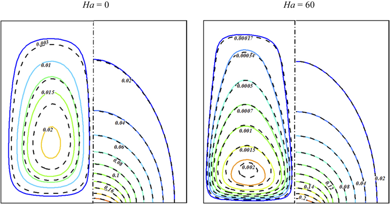
Figure 6.70 Effects of viscosity parameter [δ * = 1 (−−−) and δ * = 0 (––)] and Hartmann number on isotherms (right) and streamlines (left) when φ = 0.04, Ra = 103.

Figure 6.71 Effects of viscosity parameter [δ * = 1 (−−−) and δ * = 0 (––)] and Hartmann number on isotherms (right) and streamlines (left) when φ = 0.04, Ra = 104.
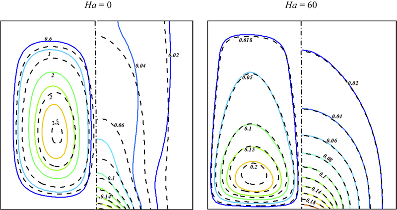
Figure 6.72 Effects of viscosity parameter [δ * = 1 (−−−) and δ * = 0 (––)] and Hartmann number on isotherms (right) and streamlines (left) when φ = 0.04, Ra = 105.
The effects of Hartmann number and Rayleigh number on local and average Nusselt number are shown in Figs. 6.73 and 6.74. Increasing Rayleigh number leads the Nusselt number to enhance. Increasing Lorentz forces make thermal boundary layer thickness to increase and in turn Nusselt number decreases with the enhancement of Hartmann number. Fig. 6.75 depicts the effect of Hartmann number and Rayleigh number on Nusselt number ratio. As viscosity parameter increases, the rate of heat transfer decreases. This reduction is more pronounced for higher values of Rayleigh number and lower values of Hartmann number. It is an interesting observation that increasing Lorentz forces increase the effect of MFD viscosity of Nusselt number. At low Rayleigh number, considering MFD viscosity has no significant effect on Nusselt number.
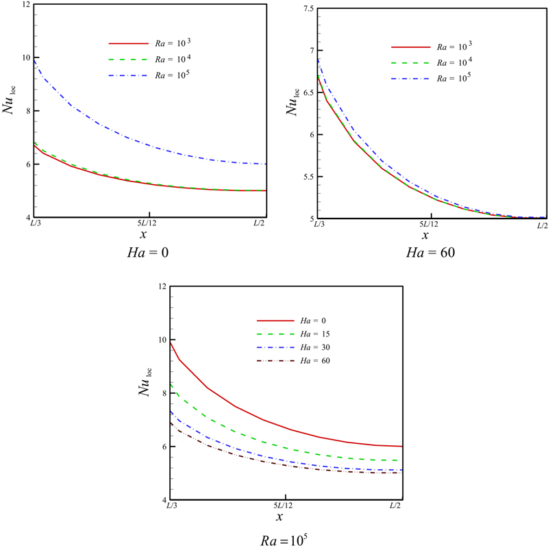
Figure 6.73 Effects of Hartmann number and Rayleigh number on local Nusselt number when φ = 0.04, δ * = 1, Pr = 6.2.
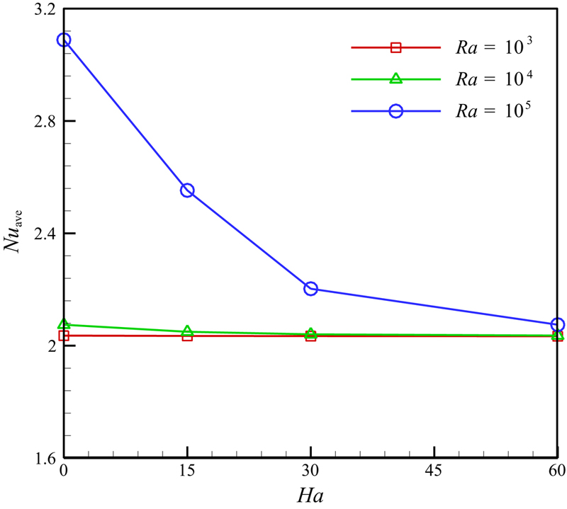
Figure 6.74 Effects of Hartmann number and Rayleigh number on average Nusselt number when φ = 0.04, δ * = 1, Pr = 6.2.

Figure 6.75 Effects of Hartmann number and Rayleigh number on Nusselt number ratio when φ = 0.04, Pr = 6.2.
..................Content has been hidden....................
You can't read the all page of ebook, please click here login for view all page.