
A time aware layer provides valuable information about the data—the entire set of values for the features at each time stop for each feature. Until now, we have been visualizing the entire spatial dataset at different time zones using a Time Slider or a similar approach in D3. We have never been able to visualize the values for a particular feature across the entire time extent, or at least across multiple time extents. Our objective in this section would be just that—to visualize the values of a selected feature across the entire time extent.
We will be using the following layer for our visualization purposes, available at http://earthobs1.arcgis.com/arcgis/rest/services/US_Drought_by_County/FeatureServer/0.
This layer shows the USA Drought intensity from 2000 to the present by county. The temporal range of data is 01/04/2000 to the present and is updated every Thursday to reflect the conditions occurring the previous week.
Our objective is to pull all the data for a selected feature. The following steps can be followed to arrive at our objective:
- Select a feature and perform an identify task on it to get the feature ID.
- Use the feature ID to query the previous feature layer.
- Pass the data to Cedar charts of the type
time.
The following piece of code explains how identify parameters are formed. The identify task is performed at each map click:
  function initIdentify () {
            map.on("click", doIdentify);

            identifyTask = new IdentifyTask("http://server.arcgisonline.com/arcgis/rest/services/Demographics/USA_1990-2000_Population_Change/MapServer");

            identifyParams = new IdentifyParameters();
            identifyParams.tolerance = 1;
            identifyParams.layerIds = [3];
            identifyParams.returnGeometry = true;
            identifyParams.layerOption = IdentifyParameters.LAYER_OPTION_ALL;
            identifyParams.width = map.width;
            identifyParams.height = map.height;
    }
The map click event calls the following function named doIdentify():
function doIdentify (event) {
      map.graphics.clear();

//Use the map click point for the identify task

      identifyParams.geometry = event.mapPoint;
      identifyParams.mapExtent = map.extent;
      identifyTask.execute(identifyParams, function (results) {
      console.log(results[0].feature.attributes);

//Initiate a Query Task

      var queryTask = new QueryTask("http://earthobs1.arcgis.com/arcgis/rest/services/US_Drought_by_County/FeatureServer/0");
      var query = new Query();
      query.returnGeometry = true;
      query.outFields = ["*"];

//Query based on the feature id returned by the identify task

      query.where = "countycategories_admin_fips = '"+results[0].feature.attributes.ID+"'";
      query.orderByFields = ["countycategories_date"];
      queryTask.execute(query).then(function(qresult){
      console.log(qresult);

//Send the query result to the topic "some/topic"

      topic.publish("some/topic", qresult);
    });
  });
}
The topic that sends the query data shall be subscribed by the function that will construct the Cedar chart. The Cedar chart type required is time.
The time type Cedar chart expects the following types of fields in the field mapping:
- Esri date time field
- Any numerical value
In our case, we will map the fields, namely countycategories_date (date time field) and countycategories_d0 (numeric field):
topic.subscribe("some/topic", function () {
            var data = arguments[0];
            var chart = new Cedar({
                "type": "time"
            });
            var dataset = {
                "data": data,
                "mappings": {
                    "time": {
                        "field": "countycategories_date",
                        "label": "Date"
                    },
                    "value": {
                        "field": "countycategories_d0",
                        "label": "Countycategories D0"
                    },
                    "sort": "countycategories_date"
                }
            };

//tool tip field
            chart.tooltip = {
                "title": "Countycategories D0",
                "content": "{countycategories_d0}"
            };


        chart.dataset = dataset;

//show the chart

chart.show({
            elementId: "#droughtHistoryMap",
            autolabels: true,
            height:150,
            width:800
        });
        chart.on('click', function(event,data){
            console.log(event,data);
            topic.publish("application/d3slider/timeChanged", new Date(data.countycategories_date));
        });
    });
Incorporating the previous code into the application, we were able to see the time-based graph of the drought values over a period for a selected county. In the following image, the graph represents the timeline of drought values for the selected feature:
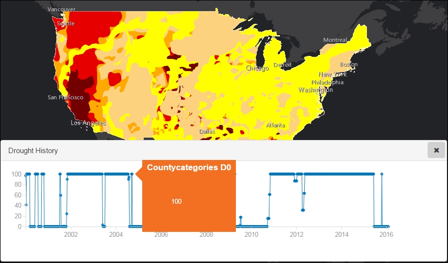
This representation gives a multidimensional perspective in more than one way. One is that we are still seeing the spatial distribution of drought for the entire country at a particular instance of time. At the same time, we are able to use a non-spatial visualization aid, such as a time-graph, to visualize the entire set of drought values throughout a time period for a particular feature at county level.