Chapter 7
Models and Clocks
7.1 Introduction
Distributed software requires a set of tools and techniques different from that required by the traditional sequential software. One of the most important issues in reasoning about a distributed program is the model used for a distributed computation. It is clear that when a distributed program is executed, at the most abstract level, a set of events is generated. Some examples of events are the beginning and the end of the execution of a function, and the sending and receiving of a message. This set alone does not characterize the behavior. We also impose an ordering relation on this set. The first relation is based on the physical time model. Assuming that all events are instantaneous, that no two events are simultaneous, and that a shared physical clock is available, we can totally order all the events in the system. This is called the interleaving model of computation. If there is no shared physical clock, then we can observe a total order among events on a single processor but only a partial order between events on different processors. The order for events on different processors is determined on the basis of the information flow from one processor to another. This is the happened-before model of a distributed computation. We describe these two models in this chapter.
In this chapter we also discuss mechanisms called clocks that can be used for tracking the order relation on the set of events. The first relation we discussed on events imposes a total order on all events. Because this total order cannot be observed, we describe a mechanism to generate a total order that could have happened in the system (rather than the one that actually happened in the system). This mechanism is called a logical clock. The second relation, happened-before, can be accurately tracked by a vector clock. A vector clock assigns timestamps to states (and events) such that the happened-before relationship between states can be determined by using the timestamps.
7.2 Model of a Distributed System
We take the following characteristics as the defining ones for distributed systems:
• Absence of a shared clock: In a distributed system, it is impossible to synchronize the clocks of different processors precisely due to uncertainty in communication delays between them. As a result, it is rare to use physical clocks for synchronization in distributed systems. In this book we will see how the concept of causality is used instead of time to tackle this problem.
• Absence of shared memory: In a distributed system, it is impossible for any one processor to know the global state of the system. As a result, it is difficult to observe any global property of the system. In this book we will see how efficient algorithms can be developed for evaluating a suitably restricted set of global properties.
• Absence of accurate failure detection: In an asynchronous distributed system (a distributed system is asynchronous if there is no upper bound on message delays), it is impossible to distinguish between a slow processor and a failed processor. This leads to many difficulties in developing algorithms for consensus, election, and so on. In this book we will see these problems, and their solutions when synchrony is assumed.
Our model for a distributed system is based on message passing, and all of our algorithms are based around that concept. Our algorithms do not assume any upper bound on the message delays. Thus we assume asynchronous systems. An advantage is that all the algorithms developed in this model are also applicable to synchronous systems.
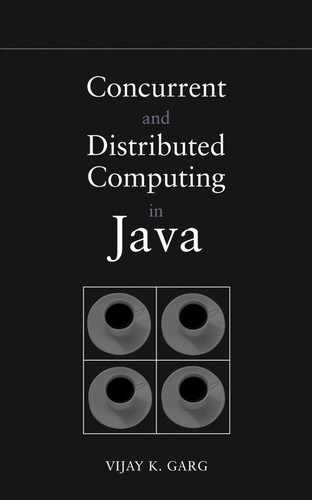
We model a distributed system as an asynchronous message-passing system without any shared memory or a global clock. A distributed program consists of a set of N processes denoted by {P1, P2, ..., PN} and a set of unidirectional channels. A channel connects two processes. Thus the topology of a distributed system can be viewed as a directed graph in which vertices represent the processes and the edges represent the channels. Figure 7.1 shows the topology of a distributed system with three processes and four channels. Observe that a bidirectional channel can simply be modeled as two unidirectional channels.
Figure 7.1: An example of topology of a distributed system
A channel is assumed to have infinite buffer and to be error-free. We do not make any assumptions on the ordering of messages. Any message sent on the channel may experience arbitrary but finite delay. The state of the channel at any point is defined to be the sequence of messages sent along that channel but not received.
A process is defined as a set of states, an initial condition (i.e., a subset of states), and a set of events. Each event may change the state of the process and the state of at most one channel incident on that process. The behavior of a process with finite states can be described visually with state transition diagrams. Figure 7.2 shows the state transition diagram for two processes. The first process P1 sends a token to P2 and then receives a token from P2. Process P2 first receives a token from P1 and then sends it back to P1. The state s1 is the initial state for P1, and the state t1 is the initial state for P2.

Figure 7.2: A simple distributed program with two processes
7.3 Model of a Distributed Computation
In this section, we describe the interleaving and the happened-before models for capturing behavior of a distributed system.
7.3.1 Interleaving Model
In this model, a distributed computation or a run is simply a global sequence of events. Thus all events in a run are interleaved. For example, consider a system with two processes: a bank server and a bank customer. The program of the bank customer process sends two request messages to the bank server querying the savings and the checking accounts. On receiving the response, it adds up the total balance. In the interleaving model, a run may be given as follows:
P1 sends “what is my checking balance” to P2
P1 sends “what is my savings balance” to P2
P2 receives “what is my checking balance” from P1
P1 sets total to 0
P2 receives “what is my savings balance” from P1
P2 sends “checking balance = 40” to P1
P1 receives “checking balance = 40” from P2
P2 sets total to 40 (total + checking balance)
P1 sends “savings balance = 70” to P2
P1 receives “savings balance = 70” from P2
P1 sets total to 110 (total + savings balance)
7.3.2 Happened-Before Model
In the interleaving model, there is a total order defined on the set of events. Lamport has argued that in a true distributed system only a partial order, called a happened-before relation, can be determined between events. In this section we define this relation formally.
As before, we will be concerned with a single computation of a distributed program. Each process Pi in that computation generates a sequence of events. It is clear how to order events within a single process. If event e occurred before f in the process, then e is ordered before f. How do we order events across processes? If e is the send event of a message and f is the receive event of the same message, then we can order e before f. Combining these two ideas, we obtain the following definition.
Definition 7.1 (Happened Before Relation) The happened-before relation. (→) is the smallest relation that satisfies
1. If e occurred before f in the same process, then e → f .
2. If e is the send event of a message and f is the receive event of the same message, then e → f.
3. If there exists an event g such that (e → g) and (g → f), then (e → f) .
In Figure 7.3, e2 → e4, e3 → f3, and e1 → g4.
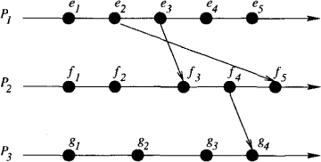
Figure 7.3: A run in the happened-before model
A run or a computation in the happened-before model is defined as a tuple (E, →) where E is the set of all events and → is a partial order on events in E such that all events within a single process are totally ordered. Figure 7.3 illustrates a run. Such figures are usually called space-time diagrams, process-time diagrams, or happened-before diagrams. In a process-time diagram, e → f iff it contains a directed path from the event e to event f . Intuitively, this relation captures the order that can be determined between events. The important thing here is that the happened-before relation is only a partial order on the set of events. Thus two events e and f may not be related by the happened-before relation. We say that e and f are concurrent (denoted by e||f) if ¬(e → f) ∧ ¬(f → e). In Figure 7.3, e2||f2, and e1||g3.
Instead of focusing on the set of events, one can also define a computation based on the the set of states of processes that occur in a computation, say S. The happened-before relation on S can be defined in the manner similar to the happened-before relation on E.
7.4 Logical Clocks
We have defined two relations between events based on the global total order of events, and the happened-before order. We now discuss mechanisms called clocks that can be used for tracking these relations.
When the behavior of a distributed computation is viewed as a total order, it is impossible to determine the actual order of events in the absence of accurately synchronized physical clocks. If the system has a shared clock (or equivalently, precisely synchronized clocks), then timestamping the event with the clock would be sufficient to determine the order. Because in the absence of a shared clock the total order between events cannot be determined, we will develop a mechanism that gives a total order that could have happened instead of the total order that did happen.
The purpose of our clock is only to give us an order between events and not any other property associated with clocks. For example, on the basis of our clocks one could not determine the time elapsed between two events. In fact, the number we associate with each event will have no relationship with the time we have on our watches.
As we have seen before, only two kinds of order information can be determined in a distributed system—the order of events on a single process and the order between the send and the receive events of a message. On the basis of these considerations, we get the following definition.
A logical clock C is a map from the set of events E to N (the set of natural numbers) with the following constraint:
∀e, f ∈ E: e → f ⇒ C(e) < C(f)
Sometimes it is more convenient to timestamp states on processes rather than events. The logical clock C also satisfies
∀s, t ∈ S: s → t ⇒ C(s) < C(t)
The constraint for logical clocks models the sequential nature of execution at each process and the physical requirement that any message transmission requires a nonzero amount of time.
Availability of a logical clock during distributed computation makes it easier to solve many distributed problems. An accurate physical clock clearly satisfies the above mentioned condition and therefore is also a logical clock. However, by definition of a distributed system there is no shared clock in the system. Figure 7.4 shows an implementation of a logical clock that does not use any shared physical clock or shared memory.
It is not required that message communication be ordered or reliable. The algorithm is described by the initial conditions and the actions taken for each event type. The algorithm uses the variable c to assign the logical clock. The notation s.c denotes the value of c in the state s. Let s.p denote the process to which state s belongs.
For any send event, the value of the clock is sent with the message and then incremented at line 14. On receiving a message, a process takes the maximum of its own clock value and the value received with the message at line 17. After taking the maximum, the process increments the clock value. On an internal event, a process simply increments its clock at line 10.
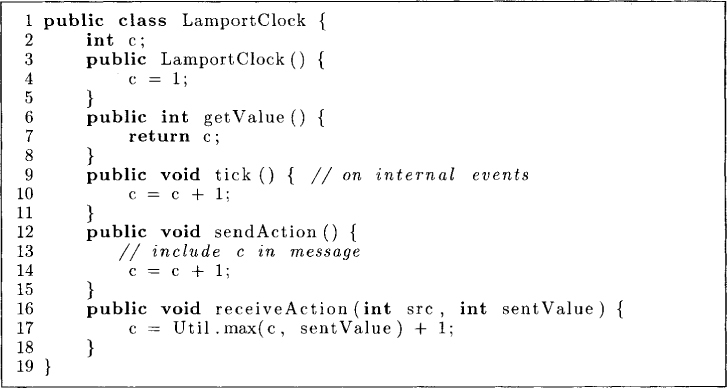
Figure 7.4: A logical clock algorithm
The following claim is easy to verify.
∀s, t ∈ S: s → t ⇒ s.c < t.c
In some applications it is required that all events in the system be ordered totally. If we extend the logical clock with the process number, then we get a total ordering on events. Recall that for any state s, s.p indicates the identity of the process to which it belongs. Thus the timestamp of any event is a tuple (s.c, s.p) and the total order < is obtained as
7.5 Vector Clocks
We saw that logical clocks satisfy the following property:
s → t ⇒ s.c < t.c
However, the converse is not true; s.c < t.c does not imply that s → t. The computation (S, →) is a partial order, but the domain of logical clock values (the set of natural numbers) is a total order with respect to <. Thus logical clocks do not provide complete information about the happened-before relation. In this section, we describe a mechanism called a vector clock that allows us to infer the happened-before relation completely.
Definition 7.2 (Vector Clock) A vector clock v is a map from S to Nk (vectors of natural numbers) with the following constraint
∀s, t : s → ⇔ s.v < t.v.
where s.v is the vector assigned to the state s.
Because → is a partial order, it is clear that the timestamping mechanism should also result in a partial order. Thus the range of the timestamping function cannot be a total order like the set of natural numbers used for logical clocks. Instead, we use vectors of natural numbers. Given two vectors x and y of dimension N, we compare them as follows:
It is clear that this order is only partial for N ≥ 2. For example, the vectors (2, 3, 0) and (0, 4, 1) are incomparable. A vector clock timestamps each event with a vector of natural numbers.
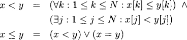
Our implementation of vector clocks uses vectors of size N, the number of processes in the system. The algorithm presented in Figure 7.5 is described by the initial conditions and the actions taken for each event type. A process increments its own component of the vector clock after each event. Furthermore, it includes a copy of its vector clock in every outgoing message. On receiving a message, it updates its vector clock by taking a componentwise maximum with the vector clock included in the message. This is shown in the method receiveAction. It is not required that message communication be ordered or reliable. A sample execution of the algorithm is given in Figure 7.7.
Figure 7.6 extends the Linker class (defined in Chapter 6) to automatically include the vector clock in all outgoing messages and to take the receiveAction when a message is received. The method sendMsg prefixes the message with the tag “vector” and the vector clock. The method simpleSendMsg is useful for application messages that do not use vector clocks. The method receiveMsg determines whether the message has a vector clock in it. If it does, the method removes the vector clock, invokes receiveAction, and then returns the application message.
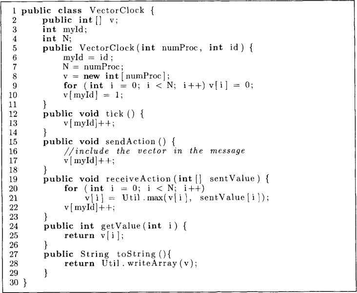
Figure 7.5: A vector clock algorithm
Figure 7.6: The VCLinker class that extends the Linker class

Figure 7.7: A sample execution of the vector clock algorithm
We now show that s → t iff s.v < t.v. We first claim that if s ≠ t, then
s ↛ t ⇒ t.v[s.p] < s.v[s.p] (7.1)
If t.p = s.p, then it follows that t occurs before s. Because the local component of the vector clock is increased after each event, t.v[s.p] < s.v[s.p]. So, we assume that s.p ≠ t.p. Since s.v[s.p] is the local clock of Ps.p, and Pt.p could not have seen this value as s ↛, t, it follows that t.v[s.p] < s.v[s.p]. Therefore, we have that (s ↛ t) implies ¬(s.v < t.v).
Now we show that (s → t) implies (s.v < t.v). If s → t, then there is a message path from s to t. Since every process updates its vector on receipt of a message and this update is done by taking the componentwise maximum, we know that the following holds:
∀k : s.v[k ≤ t.v[k].
Furthermore, since t ↛ s, from Equation (7.1), we know that s.v[t.p] is strictly less than t.v[t.p]. Hence, (s → t) ⇒ (s.v < t.v).
It is left as an exercise to show that if we know the processes the vectors came from, the comparison between two states can be made in constant time:
s → t ⇔ (s.v[s.p] ≤ t.v[s.p]) ∧ (s.v[t.p] < t.v[t.p])
7.6 Direct-Dependency Clocks
One drawback with the vector clock algorithm is that it requires O(N) integers to be sent with every message. For many applications, a weaker version of the clock suffices. We now describe a clock algorithm that is used by many algorithms in distributed systems. These clocks require only one integer to be appended to each message. We call these clocks direct-dependency clocks.
The algorithm shown in Figure 7.8 is described by the initial conditions and the actions taken for each event type. On a send event, the process sends only its local component in the message. It also increments its component as in vector clocks. The action for internal events is the same as that for vector clocks. When a process receives a message, it updates two components—one for itself, and the other for the process from which it received the message. It updates its own component in a manner identical to that for logical clocks. It also updates the component for the sender by taking the maximum with the previous value.
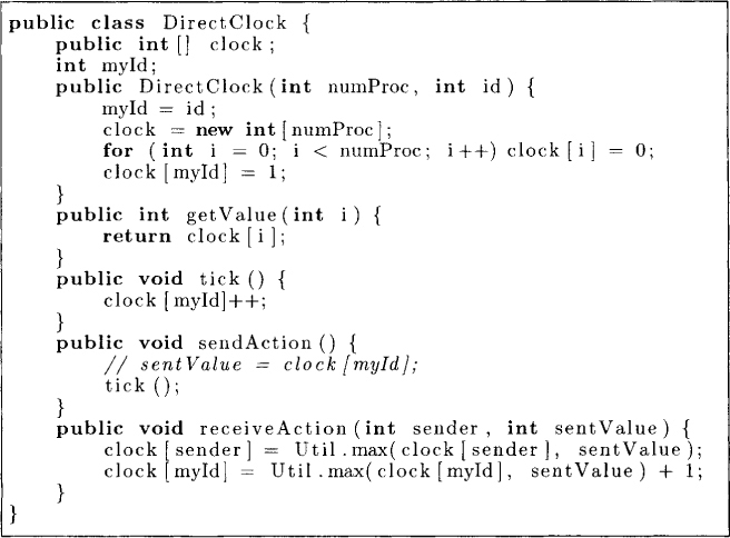
Figure 7.8: A direct-dependency clock algorithm
An example of a distributed computation and its associated direct-dependency clock is given in Figure 7.9.
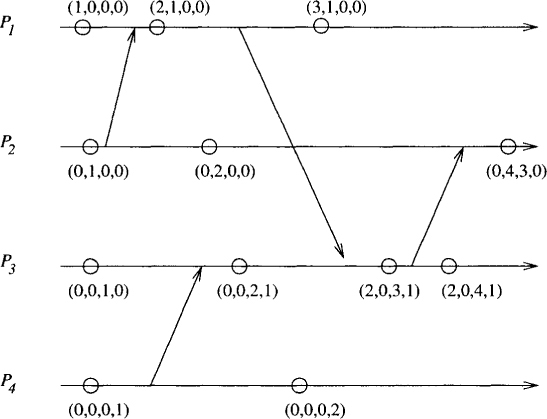
Figure 7.9: A sample execution of the direct-dependency clock algorithm.
We first observe that if we retain only the ith component for the ith process, then the algorithm above is identical to the logical clock algorithm. However, our interest in a direct-dependency clock is not due to its logical clock property (Lamport’s logical clock is sufficient for that), but to its ability to capture the notion of direct dependency. We first define a relation, directly precedes (→d), a subset of →, as follows: s →d t iff there is a path from s to t that uses at most one message in the happened-before diagram of the computation. The following property makes direct-dependency clocks useful for many applications:
∀s, t : s.p ≠ t.p : (s →d t) ⇔ (s.v[s.p] ≤ t.v[s.p])
The proof of this property is left as an exercise. The reader will see an application of direct-dependency clock in Lamport’s mutual exclusion algorithm discussed in Chapter 8.

Figure 7.10: The matrix clock algorithm
7.7 Matrix Clocks
It is natural to ask whether using higher-dimensional clocks can give processes additional knowledge. The answer is “yes.” A vector clock can be viewed as a knowledge vector. In this interpretation, s.v[i] denotes what process s.p knows about process i in the local state s. In some applications it may be important for the process to have a still higher level of knowledge. The value s.v[i, j] could represent what process s.p knows about what process i knows about process j. For example, if s.v[i, s.p] > k for all i, then process s.p can conclude that everybody knows that its state is strictly greater than k.
Next, we discuss the matrix clock that encodes a higher level of knowledge than a vector clock. The matrix clock algorithm is presented in Figure 7.10. The following description applies to an N × N matrix clock in a system with N processes. The algorithm is easier to understand by noticing the vector clock algorithm embedded within it. If we focus only on row myId for process PmyId, the algorithm presented above reduces to the vector clock algorithm. Consider the update of the matrix in the algorithm in Figure 7.10 when a message is received. The first step affects only rows different from myId and can be ignored. When a matrix is received from process srcld, then we use only the row given by the index srcId of the matrix W for updating row myId of PmyId. Thus, from our discussion of vector clock algorithms, it is clear that
∀s, t : s.p ≠ t.p : s → t ≡ s.M[s.p,.] < t.M[t.p,.]
The other rows of the matrix M keep the vector clocks of other processes. Note that initially M contains 0 vector for other processes. When it receives a matrix in W, it updates its information about the vector clock by taking componentwise maximum.
We now show an application of matrix clocks in garbage collection. Assume that a process Pi generated some information when its matrix clock value for M[i][i] equals k. Pi sends this information directly (or indirectly) to all processes and wants to delete this information when it is known to all processes. We claim that Pi can delete the information when the following condition is true for the matrix M:
∀j: M[j][i] ≥ k
This condition implies that the vector clock of all other processes j have ith component at least k. Thus, if the information is propagated through messages, Pi knows that all other processes have received the information that Pi had when M[i][i] was k.
We will later see another application of a variant of matrix clock in enforcing causal ordering of messages discussed in Chapter 12.
7.8 Problems
7.1. Give advantages and disadvantages of a parallel programming model over a distributed system (message based) model.
7.2. Show that “concurrent with” is not a transitive relation.
7.3. Write a program that takes as input a distributed computation in the happened-before model and outputs all interleavings of events that are compatible with the happened-before model.
7.4. We discussed a method by which we can totally order all events within a system. If two events have the same logical time, we broke the tie using process identifiers. This scheme always favors processes with smaller identifiers. Suggest a scheme that does not have this disadvantage. (Hint: Use the value of the logical clock in determining the priority.)
7.5. Prove the following for vector clocks: s → t iff
(s.v[s.p] ≤ t.v[s.p]) ∧ (s.v[t.p] < t.v[t.p]).
7.6. Suppose that the underlying communication system guarantees FIFO ordering of messages. How will you exploit this feature to reduce the communication complexity of the vector clock algorithm? Give an expression for overhead savings if your scheme is used instead of the traditional vector clock algorithm. Assume that any process can send at most m messages.
7.7. Assume that you have implemented the vector clock algorithm. However, some application needs Lamport’s logical clock. Write a function convert that takes as input a vector timestamp and outputs a logical clock timestamp.
7.8. Give a distributed algorithm to maintain clocks for a distributed program that has a dynamic number of processes. Assume that there are the following events in the life of any process: start-process, internal, send, receive, fork, join processid, terminate. It should be possible to infer the happened-before relation using your clocks.
7.9. Prove the following for direct-dependency clocks:
∀s, t : s.p ≠ t.p : (s →d t) ⇔ (s.v[s.p] ≤ t.v[s.p])
7.10. Show that for matrix clocks, the row corresponding to the index s.p is bigger than any other row in the matrix s.M for any state s.
7.9 Bibliographic Remarks
The idea of logical clocks is from Lamport [Lam78]. The idea of vector clocks in pure form first appeared in papers by Fidge and Mattern [Fid89, Mat89]. However, vectors had been used before in some earlier papers (e.g., [SY85]). Direct-dependency clocks have been used in mutual exclusion algorithms (e.g., [Lam78]), global property detection (e.g., [Gar96]), and recovery in distributed systems. Matrix clocks have been used for discarding obsolete information [SL87] and for detecting relational global predicates [TG93].