Chapter 11

Detecting Termination and Deadlocks

11.1 Introduction

Termination and deadlocks are crucial predicates in a distributed system. Generally, computations are expected to terminate and be free from deadlocks. It is an important problem in distributed computing to develop efficient algorithms for termination and deadlock detection. Note that both termination and deadlock are stable properties and therefore can be detected using any global snapshot algorithm. However, these predicates can be detected even more efficiently than general stable predicates. The reason for this efficiency is that these predicates are not only stable but also locally stable—the state of each process involved in the predicate does not change when the predicate becomes true. We will later define and exploit the locally stable property of the predicates to design efficient distributed algorithms.

To motivate termination detection, we consider a class of distributed computations called diffusing computations. We give a diffusing computation for the problem of determining the shortest path from a fixed process. The diffusing computation algorithm works except that one does not know when the computation has terminated.

11.2 Diffusing Computation

Consider a computation on a distributed system that is started by a special process called environment. This process starts up the computation by sending messages to some of the processes. Each process in the system is either passive or active. It is assumed that a passive process can become active only on receiving a message (an active process can become passive at any time). Furthermore, a message can be sent by a process only if it is in the active state. Such a computation is called a diffusing computation. Algorithms for many problems such as computing the breadth-first search-spanning tree in an asynchronous network or determining the shortest paths from a processor in a network can be structured as diffusing computations.

We use a distributed shortest-path algorithm to illustrate the concepts of a diffusing computation. Assume that we are interested in finding the shortest path from a fixed process called a coordinator (say, P₀) to all other processes. Each process initially knows only the average delay of all its incoming links in the array edgeWeight. A diffusing computation to compute the shortest path is quite simple. Every process P_i maintains the following variables:

1. cost: represents the cost of the shortest path from the coordinator to P_i as known to P_i currently

2. parent: represents the predecessor of P_i in the shortest path from the coordinator to P_i as known to P_i currently

The coordinator acts as the environment and starts up the diffusing computation by sending the cost of the shortest path to be 0 using a message type path. Any process P_i that receives a message from P_j of type path with cost c determines whether its current cost is greater than the cost of reaching P_j plus the cost of reaching from P_j to P_i. If that is indeed the case, then P_i has discovered a path of shorter cost and it updates the cost and parent variables. Further, any such update results in messages to its neighbors about its new cost. The algorithm is shown in Figure 11.1. Each process calls the method initiate to start the program. This call results in the coordinator sending out messages with cost 0. The method handleMsg simply handles messages of type path.

The algorithm works fine with one catch. No process ever knows when it is done, that is, the cost variable will not decrease further. In this chapter, we study how we can extend the computation to detect termination. Figure 11.2 shows the interface implemented by the termination detection algorithm. Any application which uses a TermDetector must invoke initiate at the beginning of the program, sendAction on sending a message, and turnPassive on turning passive.

From properties of a diffusing computation, it follows that if all processes are passive in the system and there are no messages in transit, then the computation has terminated. Our problem is to design a protocol by which the environment process can determine whether the computation has terminated. Our solution is based on an algorithm by Dijkstra and Scholten.

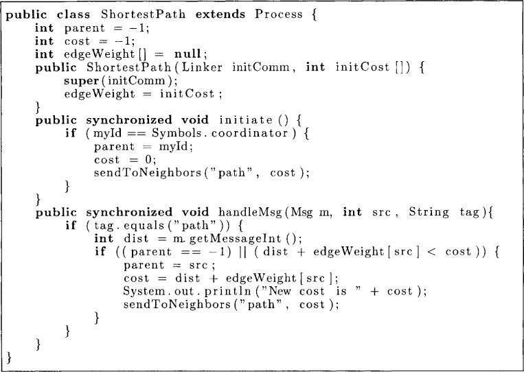
Figure 11.1: A diffusing computation for the shortest path

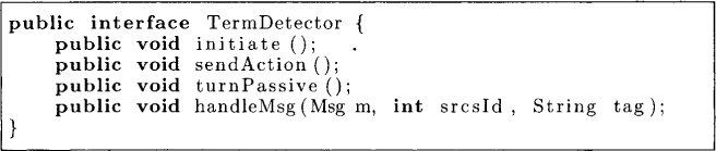
Figure 11.2: Interface for a termination detection algorithm

11.3 Dijkstra and Scholten’s Algorithm

We say that a process is in a green state if it is passive and all of its outgoing channels are empty; otherwise, it is in a red state. How can a process determine whether its outgoing channel is empty? This can be done if the receiver of the channel signals the sender of the channel the number of messages received along that channel. If the sender keeps a variable D[i] (for deficit) for each outgoing channel i, which records the number of messages sent minus the number of messages that have been acknowledged via signals, it can determine that the channel i is empty by checking whether D[i] = 0. Observe that D[i] ≥ 0 is always true. Therefore, if 0 is the set of all outgoing channels, it follows that

∀i ∈ O : D[i] = 0

is equivalent to

Thus it is sufficient for a process to maintain just one variable D that represents the total deficit for the process.

It is clear that if all processes are in the green state, then the computation has terminated. To check this condition, we will maintain a set T with the following invariant (10):

(10) All red processes are part of the set T.

Observe that green processes may also be part of T—the invariant is that there is no red process outside T. When the set T becomes empty, termination is true.

When the diffusing computation starts, the environment is the only red process initially (with nonempty outgoing channels); the invariant is made true by keeping environment in the set T. To maintain the invariant that all red processes are in T, we use the following rule. If P_j turns P_k red (by sending a message), and P_k is not in T, then we add P_k to T.

We now induce a directed graph (T, E) on the set T by defining the set of edges E as follows. We add an edge from P_j to P_k, if P_j was responsible for addition of P_k to the set T. We say that P_j is the parent of P_k. From now on we use the terms node and process interchangeably. Because every node (other than the enviromnent) has exactly one parent and an edge is drawn from P_j to P_k only when P_k is not part of T, the edges E form a spanning tree on T rooted at the environment. Our algorithm will maintain this as invariant:

(11) The edges E form a spanning tree of nodes in T rooted at the environment.

Up to now, our algorithm only increases the size of T. Because detection of termination requires the set to be empty, we clearly need a mechanism to remove nodes from T. Our rule for removal is simple—a node is removed from T only if it is a green-leaf node. When a node is removed from T, the incoming edge to that node is also removed from E. Thus the invariants (10) and (11) are maintained by this rule. To implement this rule, a node needs to keep track of the number of its children in T. This can be implemented by keeping a variable at each node numchild initialized to 0 that denotes the number of children it has in T. Whenever a new edge is formed, the child reports this to the parent by a special acknowledgment that also indicates that a new edge has been formed. When a leaf leaves T, it reports this to the parent, who decrements the count. If the node has no parent (it must be the environment) and it leaves the set T, then termination is detected. By assuming that a green-leaf node eventually reports to its parent, we conclude that once the computation terminates, it is eventually detected. Conversely, if termination is detected, then the computation has indeed terminated on account of invariant (10).

Observe that the property that a node is green is not stable and hence a node, say, P_k, that is green may become active once again on receiving a message. However, because a message can be sent only by an active process, we know that some active process (which is already a part of the spanning tree) will be now responsible for the node P_k. Thus the tree T changes with time but maintains the invariant that all active nodes are part of the tree.

11.3.1 An Optimization

The algorithm given above can be optimized for the number of messages by combining messages from the reporting process and the messages for detecting whether a node is green. To detect whether an outgoing channel is empty, we assumed a mechanism by which the receiver tells the sender the number of messages it has received. One implementation could be based on control messages called signal. For every message received, a node is eventually required to send a signal message to the sender. To avoid the use of report messages, we require that a node not send the signal message for the message that made it active until it is ready to report to leave T. When it is ready to report, the signal message for the message that made it active is sent. With this constraint we get an additional property that a node will not turn green unless all its children in the tree have reported. Thus we have also eliminated the need for maintaining numchild: only a leaf node in the tree can be green. A node is ready to report when it has turned green, that is, it is passive and D = 0. The algorithm obtained after the optimization is shown in Figure 11.3.

The algorithm uses state to record the state of the process, D to record the deficit, and parent to record the parent of the process. There is no action required on initiate. The method handleMsg reduces deficit on receiving a signal message at line 15. If D becomes 0 for the environment process, then termination is detected at line 18. On receiving an application message, a node without parent sets the source of the message as the parent. In this case, no signal is sent back. This signal is sent at line 20 or line 38 when this node is passive and its D is 0. If the receiving node had a parent, then it simply sends a signal message back at line 29. The method sendAction increments the deficit and the method turnPassive changes state to passive and sends a signal to the parent if D is 0.

Now we can solve the original problem of computing the shortest path as shown in Figure 11.4.

11.4 Termination Detection without Acknowledgment Messages

Dijkstra and Scholten’s algorithm required overhead of one acknowledgment message per application message. We now present an algorithm due to Safra as described by Dijkstra which does not use acknowledgment messages. This algorithm is based on a token going around the ring. The token collects the information from all processes and determines whether the computation has terminated. The algorithm shown in Figure 11.5 requires each process to maintain the following variables:

1. state: The state of a process is either active or passive as defined earlier.

2. color: The color of a process is either white or black. If the process is white, then it has not received any message since the last visit of the token. This variable is initialized to white.

3. c: This is an integer variable maintained by each process. It records the value of the number of messages sent by the process minus the number of messages received by that process. This variable is initialized to 0.

Process P₀ begins the detection probe by sending token to the next process when it. is passive. The token consists of two fields: color and count. The color simply records if the token has seen any black process. The count records sum of all c variables seen in this round.

When a process receives the token, it keeps the token until it becomes passive. It then forwards the token to the next process, maintaining the invariants on the color of the token and the count of the token. Thus, if a black process forwards the token, the token turns black; otherwise the token keeps its color. The count variable in the token is increased by c. The process resets its own color to white after sending the token.

Figure 11.3: Termination detection algorithm

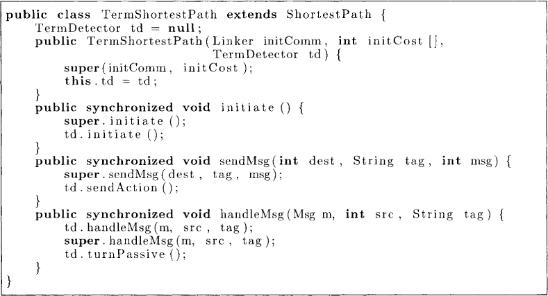
Figure 11.4: A diffusing computation for the shortest path with termination

Process P₀ is responsible for detecting termination. On receiving the token, P₀ detects termination, if its own color is white, it is passive, the token is white and the sum of token count and c is 0. If termination is not detected, then P₀ can start a new round of token passing. The correctness of this algorithm will be apparent after the discussion of locally stable predicates.

11.5 Locally Stable Predicates

We now show a technique that can be used for efficient detection of not only termination but many other locally stable predicates as well. A stable predicate B is locally stable if no process involved in the predicate can change its state relative to B once B holds. In other words, the values of all the variables involved in the predicate do not change once the predicate becomes true. The predicate B, “the distributed computation has terminated,” is locally stable. It is clear that if B is true, the states of processes will not change. Similarly, once there is a deadlock in the system the processes involved in the deadlock do not change their state.

Now consider the predicate B, “there is at most one token in the system.” This predicate is stable in a system which cannot create tokens. It is not locally stable because the state of a process can change by sending or receiving a token even when the predicate is true.

Since a locally stable predicate is also stable, one can use any global snapshot algorithm to detect it. However, computing a single global snapshot requires O(e) messages, where e is the number of unidirectional channels. We will show that for locally stable predicates, one need not compute a consistent global state.

We first generalize the notion of a consistent cut to a consistent interval. An interval is a pair of cuts (possibly inconsistent) X and Y such that X ⊆ Y. We denote an interval by [X, Y].

An interval of cuts [X, Y] is consistent if there exists a consistent cut G such that X ⊆ G ⊆ Y. Note that [G, G] is a consistent interval iff G is consistent. We now show that an interval [X, Y] is consistent iff

∀e, f : (f ∈ X) ∧ (e → f) ⇒ e ∈ Y    (11.1)

First assume that [X, Y] is a consistent interval. This implies that there exists a consistent cut G such that X ⊆ G ⊆ Y. We need to show that Equation (11.1) is true. Pick any e, f such that f ∈ X and e → f. Since f ∈ X and X ⊆ G, we get that f ∈ G. From the fact that G is consistent, we get that e ∈ G. But e ∈ G implies that e ∈ Y because G ⊆ Y. Therefore Equation (11.1) is true.

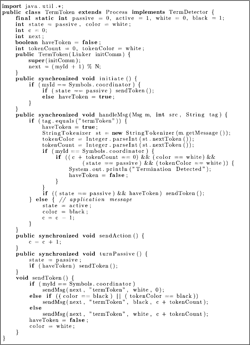
Figure 11.5: Termination detection by token traversal.

Conversely, assume that Equation (11.1) is true. We define the cut G as follows:

G = {e ∈ E| ∃f ∈ X : (e → f) ⋁ (e = f)}

Clearly, X ⊆ G from the definition of G and G ⊆ Y because of Equation (11.1). We only need to show that G is consistent. Pick any c, d such that c → d and d ∈ G. From the definition of G, there exists f ∈ X such that d = f or d + f . In either case, c → d implies that c → f and therefore c ∈ G. Hence, G is consistent.

Our algorithm will exploit the observation presented above as follows. It repeatedly computes consistent intervals [X, Y] and checks if B is true in Y and the values of variables have not changed in the interval. If both these conditions are true, then we know that there exists a consistent cut G in the interval with the same values of (relevant) variables as Y and therefore has B true. Conversely, if a predicate is locally stable and it turns true at a global state G, then all consistent intervals [X, Y] such that G ⊆ X will satisfy both the conditions checked by the algorithm.

Note that computing a consistent interval is easier than computing a consistent cut. To compute a consistent interval, we need to compute any two cuts X and Y, such that X ⊆ Y and Equation (11.1) holds. To ensure that Equation (11.1) holds, we will use the notion of barrier synchronization. Let X and Y be any cuts such that X ⊆ Y (i.e., [X, Y] is an interval) and Y has at least one event on every process. We say that an interval [X, Y] is barrier-synchronized if

∀g ∈ X ∧ h ∈ E – Y : g → h

Intuitively, this means that every event in X happened before every event that is not in Y. If [X, Y] are barrier synchronized, then they form a consistent interval. Assume, if possible, that [X, Y] is not a consistent interval. Then there exist e, f such that f ∈ X, e → f, but e ∉ Y. But e ∉ Y implies that f → e which contradicts e → f.

Barrier synchronization can be achieved in a distributed system in many ways. For example

1. P₀ sends a token to P₁ which sends it to the higher-numbered process until it reaches P_N–1. Once it reaches P_N–1, the token travels in the opposite direction. Alternatively, the token could simply go around the ring twice. These methods require every process to handle only 0(1) messages with total O(N) messages for all processes but have a high latency.

2. All processes send a message to P₀. After receiving a message from all other processes, P₀ sends a message to everybody. This method requires total O(N) messages and has a low latency but requires the coordinator to handle O(N) messages.

3. All processes send messages to everybody else. This method is symmetric and has low latency but requires O(N²) messages.

Clearly, in each of these methods a happened-before path is formed from every event before the barrier synchronization to every process after the synchronization.

Now detecting a locally stable predicate B is simple. The algorithm repeatedly collects two barrier synchronized cuts [X, Y]. If the predicate B is true in cut Y and the values of the variables in the predicate B have not changed during the interval, then B is announced to be true in spite of the fact that B is evaluated only on possibly inconsistent cuts X and Y.

11.6 Application: Deadlock Detection

We illustrate the technique for detecting locally stable predicates for deadlocks. A deadlock in a distributed system can be characterized using the wait-for graph (WFG): a graph with nodes as processes and an edge from P_i to P_j if P_i is waiting for P_j for a resource to finish its job or transaction. Thus, an edge from P_i to P_j means that there exist one or more resources held by P_j without which P_i cannot proceed. We have assumed that a process needs all the resources for which it is waiting to finish its job. Clearly, if there is a cycle in the WFG, then processes involved in the cycle will wait forever. This is called a deadlock.

A simple approach to detecting deadlocks based on the idea of locally stable predicates is as follows. We use a coordinator to collect information from processes in the system. Each process P_i maintains its local WFG, that is, all the edges in the WFG that are outgoing from P_i. It also maintains a bit changed_i, which records if its WFG has changed since its last report to the coordinator. The coordinator periodically sends a request message to all processes requesting their local WFGs. On receiving this request, a process sends its local WFG if the changed_i bit is true and “notChanged” message if changed_i is false. On receiving all local WFGs, the coordinator can combine them to form the global WFG. If this graph has a cycle, the coordinator sends a message to all processes to send their reports again. If changed_i is false for all processes involved in the cycle, then the coordinator reports deadlock.

In this algorithm, even though WFGs are constructed possibly on inconsistent global states, we know, thanks to barrier synchronization, that there exists a consistent global state with the same WFG. Therefore, any deadlock reported actually happened in a consistent global state.

We leave the Java implementation of this algorithm as an exercise.

11.7 Problems

11.1. What is the message complexity of Dijkstra and Scholten’s algorithm?

11.2. Give an algorithm based on diffusing computation to determine the breadth-first search tree from a given processor.

11.3. Extend Dijkstra and Scholten’s algorithm for the case when there can be multiple initiators of the diffusing computation.

11.4. Prove the correctness of the token-based algorithm for termination detection.

11.5. Give a Java implementation of the two-phase deadlock detection algorithm.

11.8 Bibliographic Remarks

The spanning-tree-based algorithm discussed in this chapter is a slight variant of the algorithm proposed by Dijkstra and Scholten [DS80]. The token-based termination algorithm is due to Safra as described by Dijkstra [Dij87]. The notion of locally stable predicates is due to Marzullo and Sabel [MS94]. The notion of consistent interval and the algorithm of detecting locally stable predicates by using two cuts is due to Atreya, Mittal and Garg [AMG03]. The two-phase deadlock detection algorithm is due to Ho and Ramamoorthy [HR82].