Chapter 17

Recovery

17.1 Introduction

In this chapter, we study methods for fault tolerance using checkpointing. A checkpoint can be local to a process or global in the system. A global checkpoint is simply a global state that is stored on the stable storage so that in the event of a failure the entire system can be rolled back to the global checkpoint and restarted. To record a global state, one could employ methods presented in Chapter 9. These methods, called coordinated checkpointing, can be efficiently implemented. However, there are two major disadvantages of using coordinated checkpoints:

1. There is the overhead of computing a global snapshot. When a coordinated checkpoint is taken, processes are forced to take their local checkpoints whenever the algorithm for coordinated checkpoint requires it. It is better for this decision to be local because then a process is free to take its local checkpoint whenever it is idle or the size of its state is small.

2. In case of a failure, the entire system is required to roll back. In particular, even those processes that never communicated with the process that failed are also required to roll back. This results in wasted computation and slow recovery.

An alternative method is to let processes take their local checkpoints at their will. During a failure-free mode of computation, this will result in an overhead on computation lower than that for coordinated checkpointing. In case of a failure, a suitable set of local checkpoints is chosen to form a global checkpoint. Observe that processes that have not failed have their current states available, and those states can also serve as checkpoints. There are some disadvantages of uncoordinated checkpointing compared with coordinated checkpointing schemes. First, for coordinated checkpointing it is sufficient to keep just the most recent global snapshot in the stable storage. For uncoordinated checkpoints a more complex garbage collection scheme is required. Moreover, in the case of a failure the recovery method for coordinated checkpointing is simpler. There is no need to compute a consistent global checkpoint. Finally, but most importantly, simple uncoordinated checkpointing does not guarantee any progress. If local checkpoints are taken at inopportune times, the only consistent global state may be the initial one. This problem is called the domino effect, and an example is shown in Figure 17.1. Assume that process P₁ crashes and therefore must roll back to c_1,1, its last checkpoint. Because a message was sent between c_1,1 and c_1,2 that is received before c_2.2, process P₂ is in an inconsistent state at c_2,2 with respect to Therefore, P₂ rolls back to c_2,1. But this forces P₃ to roll back. Continuing in this manner, we find that the only consistent global checkpoint is the initial one. Rolling back to the initial global checkpoint results in wasting the entire computation.

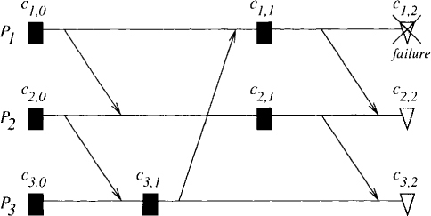
Figure 17.1: An example of the domino effect

A hybrid of the completely coordinated and the completely uncoordinated schemes is called communication-induced checkpointing. In this method, processes are free to take their local checkpoints whenever desired, but on the basis of the communication pattern, they may be forced to take additional local checkpoints. These methods guarantee that recovery will not suffer from the domino effect.

The characteristics of the application, the probability of failures, and technological factors may dictate which of the above mentioned choices of checkpointing is best for a given situation. In this chapter, we will study issues in uncoordinated checkpointing and communication-induced checkpointing.

17.2 Zigzag Relation

Consider any distributed computation with N processes P₁,. . . , P_N. Each process P_i checkpoints its local state at some intermittent interval, giving rise to a sequence of local checkpoints denoted by S_i. We will assume that the initial state and the final state in any process are checkpointed. For any checkpoint c we denote by pred.c, the predecessor of the checkpoint c in the sequence S_i whenever it exists, that is, when c is not the initial checkpoint. Similarly, we use succ.c for the successor of the checkpoint c.

Given a set of local checkpoints, X, we say that X is consistent iff ∀c, d ∈ X : c||d. A set of local checkpoints is called global if it contains N checkpoints, one from each process.

Let the set of all local checkpoints be S:

We first tackle the problem of finding a global checkpoint that contains a given set of checkpoints X ⊆ S. A relation called zigzag precedes, which is weaker (bigger) than →, is useful in analysis of such problems.

Definition 17.1 The relation zigzag precedes, denoted by , is the smallest relation that satisfies

The following property of the zigzag relation is easy to show:

On the basis of this relation, we say that a set of local checkpoints X is z-consistent iff

Observe that all initial local checkpoints c satisfy

Similarly, if c is a final local checkpoint, then

Alternatively, a zigzag path between two checkpoints c and d is defined as follows. There is a zigzag path from c to d iff

1. Both c and d are in the same process and c ≺ d; or,

2. there is a sequence of messages m₁, . . . , m_t such that

(a) m₁ is sent after the checkpoint c.

(b) If m_k is received by process r, then m_k+1 is sent by process r in the same or a later checkpoint interval. Note that the message m_k+1 may be sent before m_k.

(c) m_t is received before the checkpoint d.

In Figure 17.2, there is a zigzag path from c_1,1 to c_3,1 even though there is no happened-before path. This path corresponds to the messages m₃ and m₄ in the diagram. The message m4 is sent in the same checkpoint interval in which m₃ is received. Also note that there is a zigzag path from c_2,2 to itself because of messages m₅ and m₃. Such a path is called a zigzag cycle.

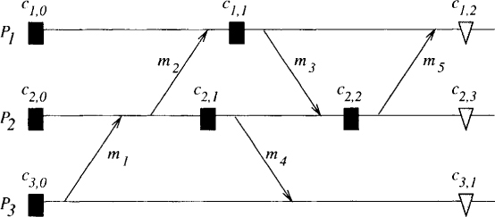
Figure 17.2: Examples of zigzag paths

We leave it as an exercise for the reader to show that iff there is a zigzag path from c to d.

We now show that given a set of local checkpoints X, there exists a consistent global checkpoint G containing X iff X is z-consistent.

We prove the contrapositive. Given c and d in X (possibly c = d), we show that implies that there is no consistent global state G containing c and d. We prove a slightly stronger claim. We show that implies that there is no consistent global state G containing c or any checkpoint preceding it and d.

The proof is based on induction on k, the minimum number of applications of rule (Z2) to derive that . When k = 0, we have c → d. Thus c or any checkpoint preceding c and d cannot be part of a consistent state by the definition of consistency. Now consider the case when because ∃e : . We show that any consistent set of states Y containing c and d cannot have any checkpoint from the process containing the checkpoint e. Y cannot contain e or any state following e because c → e would imply that c happened before that state. Furthermore, Y cannot contain any checkpoint previous to e because and the induction hypothesis would imply that Y is inconsistent. The induction hypothesis is applicable because must have fewer applications of (Z2) rule. Since any consistent set of checkpoints cannot contain any checkpoint from the process e.p, we conclude that there is no global checkpoint containing c and d.

Conversely, it is sufficient to show that if X is not global, then there exists Y strictly containing X that is z-consistent. By repeating the process, the set can be made global. Furthermore, the set is always consistent because y implies x ↛ y. For any process P_i, which does not have a checkpoint in X, we define

where min is taken over the relation ≺. Note that the set over which min is taken is nonempty because the final checkpoint on process P_i cannot zigzag precede any other checkpoint. We show that Y = X ∪ {e} is z-consistent. It is sufficient to show that and for any c in X . If e is an initial local checkpoint, then and for any c in X clearly hold. Otherwise, pred.e exists. Since e is the minimum event for which ∀x ∈ X: e ↛ x we see that there exists an event, say, d ∈ X, such that . Since and imply that , we know that is not possible. Similarly, and imply , which is false because X is z-consistent.

This result implies that if a checkpoint is part of a zigzag cycle, then it cannot be part of any global checkpoint. Such checkpoints are called useless checkpoints.

17.3 Communication-Induced Checkpointing

If a computation satisfies a condition called rollback-dependency trackability (RDT), then for every zigzag path there is also a causal path. In other words, rollback dependency is then trackable by tracking causality. Formally,

Definition 17.2 (RDT) A computation with checkpoints satisfies rollback-dependency trackability if for all checkpoints

Because there are no cycles in the happened-before relation, it follows that if a computation satisfies RDT, then it does not have any zigzag cycles. This implies that no checkpoint is useless in a computation that satisfies RDT. We now develop an algorithm for checkpointing to ensure RDT.

The algorithm takes additional checkpoints before receiving some of the messages to ensure that the overall computation is RDT. The intuition behind the algorithm is that for every zigzag path there should be a causal path. The difficulty arises when in a checkpoint interval a message is sent before another message is received. For example, in Figure 17.2 m₄ is sent before m₃ is received. When m₃ is received, a zigzag path is formed from c_1,1 to c_3,1. The message m₃ had dependency on c_1,1, which was not sent as part of m₄. To avoid this situation, we use the following rule:

Fixed dependency after send (FDAS): A process takes additional checkpoints to guarantee that the transitive dependency vector remanis unchanged after any send event (until the next checkpoint).

Thus a process takes a checkpoint before a receive of a message if it has sent a message in that checkpoint interva1 and the vector clock changes when the message is received.

A computation that uses FDAS is guaranteed to satisfy RDT because any zigzag path from checkpoints c to d implies the existence of a causal path from c to d. There are two main advantages for a computation to be RDT: (1) it allows us to calculate efficiently the maximum recoverable global state containing a given set of checkpoints (see Problem 17.2), and (2) every zigzag path implies the existence of a happened-before path. Since there are 110 cycles in the happened-before relation, it follows that the RDT graph does not have any zigzag cycles. Hence, using FDAS we can guarantee that there are no useless checkpoints in the computation.

17.4 Optimistic Message Logging: Main Ideas

In checkpointing-based methods for recovery, after a process fails, some or all of the processes roll back to their last checkpoints such that the resulting system state is consistent. For large systems, the cost of this synchronization is prohibitive. Furthermore, these protocols may not restore the maximum recoverable state.

If along with checkpoints, messages are logged to the stable storage, then the maximum recoverable state can always be restored. Theoretically, message logging alone is sufficient (assuming deterministic processes), but checkpointing speeds up the recovery. Messages can be logged by either the sender or the receiver. In pessimistic logging, messages are logged either as soon as they are received or before the receiver sends a new message. When a process fails, its last checkpoint is restored and the logged messages that were received after the checkpointed state are replayed in the order they were received. Pessimism in logging ensures that no other process needs to be rolled back. Although this recovery mechanism is simple, it reduces the speed of the computation. Therefore, it is not a desirable scheme in an environment where failures are rare and message activity is high.

In optimistic logging, it is assumed that failures are rare. A process stores the received messages in volatile memory and logs them to stable storage at infrequent intervals. Since volatile memory is lost in a failure, some of the messages cannot be replayed after the failure. Thus some of the process states are lost in the failure. States in other processes that depend on these lost states become orphans. A recovery protocol must roll back these orphan states to nonorphan states. The following properties are desirable for an optimistic recovery protocol:

• Asynchronous recovery: A process should be able to restart immediately after a failure. It should not have to wait for messages from other processes.

• Minimal amount of rollback: In some algorithms, processes that causally depend on the lost computation might roll back more than once. In the worst case, they may roll back an exponential number of times. A process should roll back at most once in response to each failure.

• No assumptions about the ordering of messages: If assumptions are made about the ordering of messages such as FIFO, then we lose the asynchronous character of the computation. A recovery protocol should make as weak assumptions as possible about the ordering of messages.

• Handle concurrent failures: It is possible that two or more processes fail concurrently in a distributed computation. A recovery protocol should handle this situation correctly and efficiently.

• Recover maximum recoverable state: No computation should be needlessly rolled back.

We present an optimistic recovery protocol that has all these features. Our protocol is based on two mechanisms—a fault-tolerant vector clock and a version end-table mechanism. The fault-tolerant vector clock is used to maintain causality information despite failures. The version end-table mechanism is used to detect orphan states and obsolete messages. In this chapter, we present necessary and sufficient conditions for a message to be obsolete and for a state to be orphan in terms of the version end-table data structure.

17.4.1 Model

In our model, processes are assumed to be piecewise deterministic. This means that when a process receives a message, it performs some internal computation, sends some messages, and then blocks itself to receive a message. All these actions are completely deterministic, that is, actions performed after a message receive and before blocking for another message receive are determined completely by the contents of the message received and the state of the process at the time of message receive. A nondeterministic action can be modeled by treating it as a message receive.

The receiver of a message depends on the content of the message and therefore on the sender of the message. This dependency relation is transitive. The receiver becomes dependent only after the received message is delivered. From now on, unless otherwise stated, receive of a message will imply its delivery.

A process periodically takes its checkpoint. It also asynchronously logs to the stable storage all messages received in the order they are received. At the time of checkpointing, all unlogged messages are also logged.

A failed process restarts by creating a new version of itself. It restores its last checkpoint and replays the logged messages that were received after the restored state. Because some of the messages might not have been logged at the time of the failure, some of the old states, called lost states, cannot be recreated. Now, consider the states in other processes that depend on the lost states. These states, called orphan states, must be rolled back. Other processes have not failed, so before rolling back, they can log all the unlogged messages and save their states. Thus no information is lost in rollback. Note the distinction between restart and rollback. A failed process restarts, whereas an orphan process rolls back. Some information is lost in restart but not in rollback. A process creates a new version of itself on restart but not on rollback. A message sent by a lost or an orphan state is called an obsolete message. A process receiving an obsolete message must discard it. Otherwise, the receiver becomes an orphan.

In Figure 17.3, a distributed computation is shown. Process P₁ fails at state f₁₀, restores state s₁₁, takes some actions needed for recovery, and restarts from state r₁₀. States s₁₂ and f₁₀ are lost. Being dependent on s₁₂, state s₂₂ of P₂ is an orphan. P₂ rolls back, restores state s₂₁, takes actions needed for recovery, and restarts from state r₂₀. Dashed lines show the lost computation. Solid lines show the useful computation at the current point.

17.4.2 Fault-Tolerant Vector Clock

Recall that a vector clock is a vector whose number of components equals the number of processes. Each entry is the timestamp of the corresponding process. To maintain causality despite failures, we extend each entry by a version number. The extended vector clock is referred to as the fault-tolerant vector clock (FTVC). We use the term “clock” and the acronym FTVC interchangeably. Let us consider the FTVC of a process P_i. The version number in the ith entry of its FTVC (its own version number) is equal to the number of times it has rolled back. The version number in the jth entry is equal to the highest version number of P_j on which P_i depends. Let entry e correspond to a tuple(version v, timestamp ts). Then, e₁ < e₂ ≡ (v₁ < v₂ ⋁ [(v₁ = v₂) ∧ (ts₁ < ts₂)].

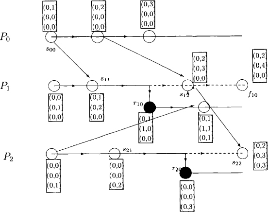
Figure 17.3: A distributed computation

A process P_i sends its FTVC along with every outgoing message. After sending a message, P_i increments its timestamp. On receiving a message, it updates its FTVC with the message’s FTVC by taking the componentwise maximum of entries and incrementing its own timestamp. To take the maximum, the entry with the higher version number is chosen. If both entries have the same version number, then the entry with the higher timestamp value is chosen.

When a process restarts after a failure or rolls back because of failure of some other process, it increments its version number and sets its timestamp to zero. Note that this operation does not require access to previous timestamps that may be lost on a failure. It requires only its previous version number. As explained in Section 17.5.2, the version number is not lost in a failure. A formal description of the FTVC algorithm is given in Figure 17.4.

An example of FTVC is shown in Figure 17.3. The FTVC of each state is shown in a rectangular box near it.

17.4.3 Version End Table

Orphan states and resulting obsolete messages are detected with the version end-table mechanism. This method requires that, after recovering from a failure, a process notify other processes by broadcasting a token. The token contains the version number that failed and the timestamp of that version at the point of restoration. We do not make any assumption about the ordering of tokens among themselves or with respect to the messages. We assume that tokens are delivered reliably.

Every process maintains some information, called vtable, about other processes in its stable storage. In vtable of P_i, there is a record for every known version of processes that ended in a failure. If P_i has received a token about kth version of P_i, then it keeps that token’s timestamp in the corresponding record in vtable. The routine insert(vtable[j], token) inserts the token in that part of the vtable of P_i that keeps track of P_j.

A formal description of the version end-table manipulation algorithm is given in Figure 17.5.

17.5 An Asynchronous Recovery Protocol

Our protocol for asynchronous recovery is shown in Figure 17.6. We describe the actions taken by a process, say, P_i, on the occurrence of different events. We assume that each action taken by a process is atomic. This means that any failure during the execution of any action may be viewed as a failure before or after the execution of the entire action.

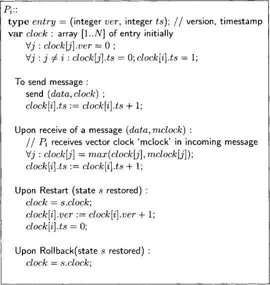
Figure 17.4: Formal description of the fault-tolerant vector clock

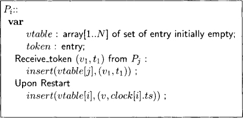
Figure 17.5: Formal description of the version end-table mechanism

17.5.1 Message Receive

On receiving a message, P_i first checks whether the message is obsolete. This is done as follows. Let e_j refer to the jth entry in the message’s FTVC. Recall that each entry is of the form (v, t), where v is the version number and t is the timestamp. If there exists an entry e_j, such that e_j is (v, t) and (v, t’) belongs to vtable[j] of P_i and t > t’, then the message is obsolete. This is proved later.

If the message is obsolete, then it is discarded. Otherwise, P_i checks whether the message is deliverable. The message is not deliverable if its FTVC contains a version number k for any process P_j, such that P_i has not received all the tokens from P_j with the version number l less than k. In this case, delivery of the message is postponed. Since we assume failures to be rare, this should not affect the speed of the computation.

If the message is delivered, then the vector clock and the version end-table are updated. P_i, updates its FTVC with the message’s FTVC as explained in Section 17.4.2. The message and its FTVC are logged in the volatile storage. Asynchronously, the volatile log is flushed to the stable storage. The version end-table is updated as explained in Section 17.4.3.

17.5.2 On Restart after a Failure

After a failure, P_i restores its last checkpoint from the stable storage (including the version end-table). Then it replays all the logged messages received after the restored state, in the receipt order. To inform other processes about its failure, it broadcasts a token containing its current version number and timestamp. After that, it increments its own version number and resets its own timestamp to zero. Finally, it updates its version end-table, takes a new checkpoint, and starts computing in a normal fashion. The new checkpoint is needed to avoid the loss of the current version number in another failure. Note that the recovery is unaffected by a failure during this checkpointing. The entire event must appear atomic despite a failure. If the failure occurs before the new checkpoint is finished, then it should appear that the restart never happened and the restart event can be executed again.

17.5.3 On Receiving a Token

We require all tokens to be logged synchronously, that is, the process is not allowed to compute further until the information about the token is in stable storage. This prevents the process from losing the information about the token if it fails after acting on it. Since we expect the number of failures to be small, this would incur only a small overhead.

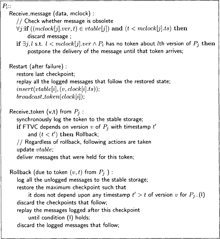
Figure 17.6: An optimistic protocol for asynchronous recovery

The token enables a process to discover whether it has become an orphan. To check whether it has become an orphan, it proceeds as follows. Assume that it received the token (v, t) from P_j. It checks whether its vector clock indicates that it depends on a state (v, t') such that. t < t'. If so, then P_i is an orphan and it needs to roll back.

Regardless of the rollback, P_i enters the record (v, t) in version end-table [j]. Finally, messages that were held for this token are delivered.

17.5.4 On Rollback

On a rollback due to token (v, t) from P_j, P_i, first logs all the unlogged messages to the stable storage. Then it restores the maximum checkpoint s such that s does not depend on any state on P_j with version number v and timestamp greater than t. Then logged messages that were received after s are replayed as long as messages are not obsolete. It discards the checkpoints and logged messages that follow this state. Now the FTVC is updated by incrementing its timestamp. Note that it does not increment its version number. After this step, P_i restarts computing as normal.

This protocol has the following properties:

• Asynchronous recovery: After a failure, a process restores itself and starts computing. It broadcasts a token about its failure, but it does not require any response.

• Minimal rollback: In response to the failure of a given version of a given process, other processes roll back at most once. This rollback occurs on receiving the corresponding token.

• Handling concurrent failures: In response to multiple failures, a process rolls back in the order in which it receives information about different failures. Concurrent failures have the same effect as that of multiple nonconcurrent failures.

• Recovering maximum recoverable state: Only orphan states are rolled back.

We now do the overhead analysis of the protocol. Except for application messages, the protocol causes no extra messages to be sent during failure-free run. It tags a FTVC to every application message. Let the maximum number of failures of any process be f. The protocol adds log f bits to each timestamp in the vector clock. Since we expect the number of failures to be small, log f should be small. Thus the total overhead is O(N log f) bits per message in addition to the vector clock.

A token is broadcast only when a process fails. The size of a token is equal to just one entry of the vector clock.

Let the number of processes in the system be n. There are at most f versions of a process, and there is one entry for each version of a process in the version end-table.

17.6 Problems

17.1. Show that the following rules are special cases of FDAS.

(a) A process takes a checkpoint before every receive of a message.

(b) A process takes a checkpoint after every send of a message.

(c) A process takes a checkpoint before any receive after any send of a message.

17.2. Assume that a computation satisfies RDT. Given a set of checkpoints X from this computation, show how you will determine whether there exists a global checkpoint containing X. If there exists one, then give an efficient algorithm to determine the least and the greatest global checkpoints containing X.

17.3. (due to Helary et al. [HMNR97]) Assume that all processes maintain a variant of logical clocks defined as follows: The logical clock is incremented on any checkpointing event. The clock value is piggybacked on every message. On receiving a message, the logical clock is computed as the maximum of the local clock and the value received with the message. Processes are free to take their local checkpoints whenever desired. In addition, a process is forced to take a local checkpoint on receiving a message if (a) it has sent out a message since its last checkpoint, and (b) the value of its logical clock will change on receiving the message. Show that this algorithm guarantees that there are no useless checkpoints. Will this protocol force more checkpoints or fewer checkpoints than the FDAS protocol?

17.4. In many applications, the distributed program may output to the external environment such that the output message cannot be revoked (or the environment cannot be rolled back). This is called the output commit problem. What changes will you make to the algorithm to take care of such messages?

17.5. Give a scheme for garbage collection of obsolete local checkpoints and message logs.

17.7 Bibliographic Remarks

The zigzag relation was first defined by Netzer and Xu [NX95]. The definition we have used in this chapter is different from but equivalent to their definition. The notion of the R-graph, RDT computation, and the fixed-dependency-after-send rule was introduced by Wang [Wan97].

Strom and Yemini [SY85] initiated the area of optimistic message logging. Their scheme, however, suffers from the exponential rollback problem, where a single failure of a process can roll back another process an exponential number of times. The algorithm discussed in this chapter is taken from a paper by Damani and Garg [DG96].