Chapter 10

Global Properties

10.1 Introduction

In this chapter, we introduce another useful tool for monitoring distributed computations. A distributed computation is generally monitored to detect if the system has reached a global state satisfying a certain property. For example, a token ring system may be monitored for the loss of the token. A distributed database system may be monitored for deadlocks. The global snapshot algorithm discussed in Chapter 9 can be used to detect a stable predicate in a distributed computation. To define stable predicates, we use the notion of the reachability of one global state from another. For two consistent global states G and H, we say that G ≤ H if H is reachable from G. A predicate B is stable iff

∀G, H : G ≤ H : B(G) ⇒ B(H)

In other words, a property B is stable if once it becomes true, it stays true. Some examples of stable properties are deadlock, termination, and loss of a token. Once a system has deadlocked or terminated, it remains in that state. A simple algorithm to detect a stable property is as follows. Compute a consistent global state. If the property B is true in that global state, then we are done. Otherwise, we repeat the process after some period of time. It is easily seen that if the stable property ever becomes true, the algorithm will detect it. Conversely, if the algorithm detects that some stable property B is true, then the property must have become true in the past (and is therefore also true currently).

Formally, if the global snapshot computation was started in the global state G_i, the algorithm finished by the global state G_f, and the recorded state is G_*, then the following is true:

1. B(G_*) ⇒ B(G_f)

2. ¬B(G_*) ⇒ ¬B(G_i)

Note that the converses of statements 1 and 2 may not hold.

At this point it is important to observe some limitations of the snapshot algorithm for detection of global properties:

• The algorithm is not useful for unstable predicates. An unstable predicate may turn true only between two snapshots.

• In many applications (such as debugging), it is desirable to compute the least global state that satisfies some given predicate. The snapshot algorithm cannot be used for this purpose.

• The algorithm may result in an excessive overhead depending on the frequency of snapshots. A process in Chandy and Lamport’s algorithm is forced to take a local snapshot on receiving a marker even if it knows that the global snapshot that includes its local snapshot cannot satisfy the predicate being detected. For example, suppose that the property being detected is termination. Clearly, if a process is not terminated, then the entire system could not have terminated. In this case, computation of the global snapshot is a wasted effort.

10.2 Unstable Predicate Detection

In this section, we discuss an algorithm to detect unstable predicates. We will assume that the given global predicate, say, B, is constructed from local predicates using boolean connectives. We first show that B can be detected using an algorithm that can detect q, where q is a pure conjunction of local predicates. The predicate B can be rewritten in its disjunctive normal form. Thus

B = q₁ ⋁ … ⋁ qk    k ≥1

where each q_i is a pure conjunction of local predicates. Next, observe that a global cut satisfies B if and only if it satisfies at least one of the q_i’s. Thus the problem of detecting B is reduced to solving k problems of detecting q, where q is a pure conjunction of local predicates.

As an example, consider a distributed program in which x, y, and z are in three different processes. Then,

even(x) ∧ ((y < 0) ⋁ (z > 6))

can be rewritten as

(even(x) ∧ (y < 0)) ⋁ (even(x) ∧ (z > 6))

where each disjunct is a conjunctive predicate.

Note that even if the global predicate is not a boolean expression of local predicates, but is satisfied by a finite number of possible global states, it can also be rewritten as a disjunction of conjunctive predicates. For example, consider the predicate (x = y), where x and y are in different processes. (x = y) is not a local predicate because it depends on both processes. However, if we know that x and y can take values {0,1} only, we can rewrite the preceding expression as follows:

((x = 0) ∧ (y = 0)) ⋁ ((x = 1) ∧ (y = 1)).

Each of the disjuncts in this expression is a conjunctive predicate.

In this chapter we study methods to detect global predicates that are conjunctions of local predicates. We will implement the interface Sensor, which abstracts the functionality of a global predicate evaluation algorithm. This interface is shown below:

public interface Sensor extends MsgHandler {
      void localPredicateTrue (VectorClock vc );
}

Any application that uses Sensor is required to call localPredicateTrue whenever its local predicate becomes true and provide its VectorClock. It also needs to implement the following interface:

public interface SensorUser extends MsgHandler {
      void globalPredicateTrue (int G[]);
      void globalPredicateFalse (int pid );
}

The class that implements Sensor calls these methods when the value of the global predicate becomes known. If the global predicate is true in a consistent global state G, then the vector clock for the global state is passed as a parameter to the method. If the global predicate is false, then the process id of the process that terminated is passed as a parameter.

We have emphasized conjunctive predicates and not disjunctive predicates. The reason is that disjunctive predicates are quite simple to detect. To detect a disjunctive predicate l₁ ⋁ l₂ ⋁ . . . ⋁ l_N, where l_i denotes a local predicate in the process P_i, it is sufficient for the process P_i to monitor l_i. If any of the processes finds its local predicate true, then the disjunctive predicate is true.

Formally, we define a weak conjunctive predicate (WCP) to be true for a given computation if and only if there exists a consistent global cut in that run in which all conjuncts are true. Intuitively, detecting a weak conjunctive predicate is generally useful when one is interested in detecting a combination of states that is unsafe. For example, violation of mutual exclusion for a two-process system can be written as “P₁ is in the critical section and P₂ is in the critical section.” It is necessary and sufficient to find a set of incomparable states, one on each process in which local predicates are true, to detect a weak conjunctive predicate. We now present an algorithm to do so. This algorithm finds the least consistent cut for which a WCP is true.

In this algorithm, one process serves as a checker. All other processes involved in detecting the WCP are referred to as application processes. Each application process checks for local predicates. It also maintains the vector clock algorithm. Whenever the local predicate of a process becomes true for the first time since the most recently sent message (or the beginning of the trace), it generates a debug message containing its local timestamp vector and sends it to the checker process.

Note that a process is not required to send its vector clock every time the local predicate is detected. If two local states, say, s and t, on the same process are separated only by internal events, then they are indistinguishable to other processes so far as consistency is concerned, that is, if u is a local state on some other process, then s||u if and only if t||u. Thus it is sufficient to consider at most one local state between two external events and the vector clock need not be sent if there has been no message activity since the last time the vector clock was sent.

The checker process is responsible for searching for a consistent cut that satisfies the WCP by considering a sequence of candidate cuts. If the candidate cut either is not a consistent cut or does not satisfy some term of the WCP, the checker can efficiently eliminate one of the states along the cut. The eliminated state can never be part of a consistent cut that satisfies the WCP. The checker can then advance the cut by considering the successor to one of the eliminated states on the cut. If the checker finds a cut for which no state can be eliminated, then that cut satisfies the WCP and the detection algorithm halts. The algorithm for the checker process is shown in Figure 10.1.

The checker receives local snapshots from the other processes in the system. These messages are used by the checker to create and maintain data structures that describe the global state of the system for the current cut. The data structures are divided into two categories: queues of incoming messages and those data structures that describe the state of the processes.

The queue of incoming messages is used to hold incoming local snapshots from application processes. We require that messages from an individual process be received in FIFO order. We abstract the message-passing system as a set of N FIFO queues, one for each process. We use the notation q[1.. . N] to label these queues in the algorithm.

Figure 10.1: WCP (weak conjunctive predicate) detection algorithm—checker process.

The checker also maintains information describing one state from each process P_i. cut[i] represents the state from P_i using the vector clock. Thus, cut[i][j] denotes the j^th component of the vector clock of cut[i]. The color[i] of a state cut[i] is either red or green and indicates whether the state has been eliminated in the current cut. A state is green only if it is concurrent with all other green states. A state is red only if it cannot be part of a consistent cut that satisfies the WCP.

The aim of advancing the cut is to find a new candidate cut. However, we can advance the cut only if we have eliminated at least one state along the current cut and if a message can be received from the corresponding process. The data structures for the processes are updated to reflect the new cut. This is done by the procedure paintState. The parameter i is the index of the process from which a local snapshot was most recently received. The color of cut[i] is temporarily set to green. It may be necessary to change some green states to red to preserve the property that all green states are mutually concurrent. Hence, we must compare the vector clock of cut[i] to each of the other green states. Whenever the states are comparable, the smaller of the two is painted red.

Let N denote the number of processes involved in the WCP and m denote the maximum number of messages sent or received by any process.

The main time complexity is involved in detecting the local predicates and time required to maintain vector clocks. In the worst case, one debug message is generated for each program message sent or received, so the worst-case message complexity is O(m). In addition, program messages have to include vector clocks.

The main space requirement of the checker process is the buffer for the local snapshots. Each local snapshot consists of a vector clock that requires O(N) space. Since there are at most O(mN) local snapshots, O(N²m) total space is required to hold the component of local snapshots devoted to vector clocks. Therefore, the total amount of space required by the checker process is O(N²m).

We now discuss the time complexity of the checker process. Note that it takes only two comparisons to check whether two vectors are concurrent. Hence, each invocation of paintState requires at most N comparisons. This function is called at most once for each state, and there are at most mN states. Therefore, at most N2m comparisons are required by the algorithm.

10.3 Application: Distributed Debugging

Assume that a programmer is interested in developing an application in which there is a leader or a coordinator at all times. Since the leader has to perform more work than other nodes, the programmer came up with the idea of circulating a token in the network and requiring that whichever node has the token acts as the leader. We will assume that this is accomplished using the class CircToken discussed in Chapter 8. Now, the programmer wants to ensure that his program is correct. He constructs the bad condition as “there is no coordinator in the system.” This condition can be equivalently written as “P₁ does not have the token, and P₂ does not have the token,” and so on for all processes. To see if this condition becomes true, the programmer must modify his program to send a vector clock to the sensor whenever the local condition “does not have the token” becomes true. Figure 10.2 shows the circulating token application modified to work with the class Sensor. Figure 10.3 shows the main application that runs the application with the sensor. This program has an additional command-line argument that specifies which sensor algorithm needs to be invoked as sensor—the centralized algorithm discussed in this section, or the distributed algorithm discussed in the next section.

When the programmer runs the program, he may discover that the global condition actually becomes true, that is, there is a global state in which there is no coordinator in the system. This simple test exposed the fallacy in the programmer’s thinking. The token may be in transit and at that time there is no coordinator in the system.

We leave it for the reader to modify the circulating token application in which a process continues to act as the leader until it receives an acknowledgment for the token. This solution assumes that the application work correctly even if there are two processes acting as the leader temporarily.

10.4 A Token-Based Algorithm for Detecting Predicates

Up to this point we have described detection of WCP on the basis of a checker process. The checker process in the vector-clock-based centralized algorithm requires O(N²m) time and space, where m is the number of messages sent or received by any process and N is the number of processes over which the predicate is defined. We now introduce token-based algorithms that distribute the computation and space requirements of the detection procedure. The distributed algorithm has O(N²m) time, space, and message complexity, distributed such that each process performs O(Nm) work.

We introduce a new set of N monitor processes. One monitor process is mated to each application process. The application processes interact according to the distributed application. In addition, the application processes send local snapshots to monitor processes. The monitor processes interact with each other but do not, send any information to the application processes.

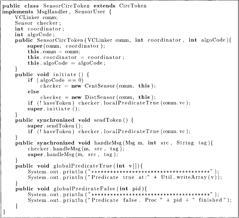
Figure 10.2: Circulating token with vector clock

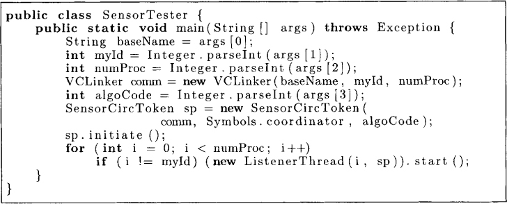
Figure 10.3: An application that runs circulating token with a sensor

The distributed WCP detection algorithm shown in Figure 10.4 uses a unique token. The token contains two vectors. The first vector is labeled G. This vector defines the current candidate cut. If G[i] has the value k, then state k from process P_i is part of the current candidate cut. Note that all states on the candidate cut satisfy local predicates. However, the states may not be mutually concurrent, that is, the candidate cut may not be a consistent cut. The token is initialized with ∀_i: G[i] = 0.

The second vector is labeled color, where color[i] indicates the color for the candidate state from application process P_i. The color of a state can be either red or green. If color[i] equals red, then the state (i, G[i]) and all its predecessors have been eliminated and can never satisfy the WCP. If color[i] = green, then there is no state in G such that (i, G[i]) happened before that state. The token is initialized with ∀_i: color[i] = red.

The token is sent to monitor process M_i only when color[i] = red. When it receives the token, M_i waits to receive a new candidate state from P_i and then checks for violations of consistency conditions with this new candidate. This activity is repeated until the candidate state does not causally precede any other state on the candidate cut, that is, the candidate can be labeled green. Next, M_i examines the token to see if any other states violate concurrency. If it finds any j such that (j, G[j]) happened before (i, G[i]) then it makes color[j] red. Finally, if all states in G are green, that is, G is consistent, then M_i has detected the WCP. Otherwise, sends the token to a process whose color is red.

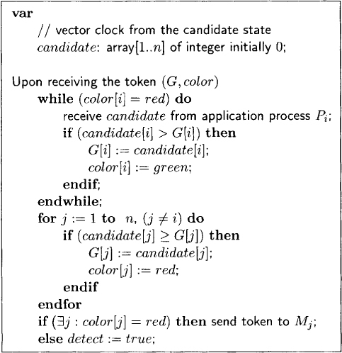
Figure 10.4: Monitor process algorithm at P_i

The implementation for the algorithm is given in Figure 10.5. It uses three types of messages. The true VC message is sent by the application process to the monitor process whenever the local predicate becomes true in a message interval. This message includes the value of the vector clock when the local predicate became true. This vector is stored in the queue q. The Token message denotes the token used in the description of the algorithm. Whenever a monitor process receives the token, it invokes the method handleToken described later. For simplicity of implementation, we send the G vector and the color vector separately. The finished message from the application process indicates that it has ended and that there will not be any more messages from it.

Let us now look at the handleToken method. The goal of the process is to make the entry color[i] green. If there is no pending vector in the queue q, then the monitor process simply waits for either a true VC or a finished message to arrive. If there is no pending vector and the finished message has been received, then we know that the global predicate can never be true and thus it is declared to be false for this computation. If a vector, candidate, is found such that candidate[i] > G[i], then the global cut is advanced to include candidate [i]. This advancement may result in color[j] becoming red if candidate[j] ≥ G[j]. The method getRed determines the first process that has red color. If the array color is completely green, getRed returns –1, and the global predicate is detected to be true. Otherwise, the token is sent to the process returned by getRed.

Let us analyze the time complexity of the algorithm. It is easy to see that whenever a process receives the token, it deletes at least one local state, that is, it receives at least one message from the application process. Every time a state is eliminated, O(N) work is performed by the process with the token. There are at most mN states; therefore, the total computation time for all processes is O(N²m). The work for any process in the distributed algorithm is at most O(Nm). The analysis of message and space complexity is left as an exercise (see Problem 10.4).

10.5 Problems

  10.1. Show that it is sufficient to send the vector clock once after each message is sent irrespective of the number of messages received.

  10.2. Assume that the given global predicate is a simple conjunction of local predicates. Further assume that the global predicate is stable. In this scenario, both Chandy and Lamport’s algorithm and the weak conjunctive algorithm can be used to detect the global predicate. What are the advantages and disadvantages of using each of them?

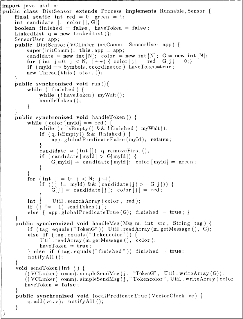
Figure 10.5: Token-based WCP detection algorithm.

  10.3. Show that if the given weak conjunctive predicate has a conjunct from each of the processes, then direct dependency clocks can be used instead of the vector clocks in the implementation of sensors. Give an example showing that if there is a process that does not have any conjunct in the global predicate, then direct dependency clocks cannot be used.

  10.4. Show that the message complexity of the vector-clock-based distributed algorithm is O(mN), the bit complexity (number of bits communicated) is O(N²m), and the space complexity is O(mN) entries per process.

  10.5. The main drawback of the single-token WCP detection algorithm is that it has no concurrency—a monitor process is active only if it has the token. Design an algorithm that uses multiple tokens in the system. [Hint: Partition the set of monitor processes into g groups and use one token-algorithm for each group. Once there are no longer any red states from processes within the group, the token is returned to a predetermined process (say, Po). When P₀ has received all the tokens, it merges the information in the g tokens to identify a new global cut. Some processes may not satisfy the consistency condition for this new cut. If so, a token is sent into each group containing such a process.]

  10.6. Design a hierarchical algorithm to detect WCP based on ideas in the previous exercise.

  10.7. Show the following properties of the vector-clock-based algorithm for WCP detection: for any i,

1. G[i] ≠ 0 ∧ color[i] = red ⇒ ∃j : j ≠ i : (i, G[i]) → (j, G[j]);

2. color[i] = green ⇒ ∀k : (i, G[i]) ↛ (k, G[k]);

3. (color[i]= green) ∧ (color[j] = green) ⇒ (i, G[i]) || (j, G[j]).

4. If (color[i] = red), then there is no global cut satisfying the WCP which includes (i, G[i]).

  10.8. Show the following claim for the vector-clock-based distributed WCP detection algorithm: The flag detect is true with G if and only if G is the smallest global state that satisfies the WCP.

*10.9. (due to Hurfin et, al.[HMRS95]) Assume that every process communicates with every other process directly or indirectly infinitely often. Design a distributed algorithm in which information is piggybacked on existing program messages to detect a conjunctive predicate under this assumption, that is, the algorithm does not use any additional messages for detection purposes.

10.6 Bibliographic Remarks

Detection of conjunctive properties was first discussed by Garg and Waldecker[GW92]. Distributed online algorithms for detecting conjunctive predicates were first presented by Garg and Chase [GC95]. Hurfin et al.[HMRS95] were the first to give a distributed algorithm that does not use any additional messages for predicate detection. Their algorithm piggybacks additional information on program messages to detect conjunctive predicates. Distributed algorithms for offline evaluation of global predicates are also discussed in Venkatesan and Dathan [VD92]. Stoller and Schneider [SS95] have shown how Cooper and Marzullo’s algorithm can be integrated with that of Garg and Waldecker to detect conjunction of global predicates. Lower bounds on these algorithms were discussed by Garg [Gar92].