
June 12, 2012 18:12 PSP Book - 9in x 6in 07-Junichi-Takeno-c07
Theory of Robot Evolution 117
For now, the four surviving robots reproduce eight robots by
mating. These eight robots are the (n + 1)th generation. The
robots of this new generation are evaluated to select the surviving
robots. At this time, the value of the fitness function increased
to more than 77. We can hopefully expect the fitness function to
increase gradually by repeating the above process generation after
generation. Repetition stops when robots of a high evaluation are
found. This is a breakthrough approach in that the details of the
artificial neural network are omitted and the overall picture is
grasped. This sounds like saying that good results are important no
matter how the artificial neural network is structured. That is why
this approach is enthusiastically hailed by behaviorists.
The machine evolution approach is said to have been initiated
by John Holland and L.J. Fogel, both in the United States, and Ingo
Rechenberg in Germany, in the 1960s almost simultaneously (Pfeifer
and Sceider, 2001). Holland advocated a genetic algorithm, while
Fogel promoted evolutionary programming, and Rechenberg de-
veloped an evolutionary strategy technique. The three researchers
seem to have been working in different fields of study, but in reality
there is no significant difference among them from the broader
perspective of machine evolution.
The machine evolution approach has made a great progress
historically hand in hand with the study of artificial life.
“Artificial life,” as defined by Christopher Langton of the Santa
Fe Institute, “is an artificial system that behaves like a living
organism.” In the study of artificial life, artificial living organisms,
called creatures, reproduce themselves, grow, prosper, decay, and die
by simulation in computers.
In their studies, artificial life researchers naturally discuss the
evolution of their artificial living organisms. However, their research
is performed in an ideal environment of computers, which is
markedly different from the environment of machine evolution
research.
Researchers of machine evolution claim that machines acquire
knowledge through interaction with the natural environment. This
very belief prevents them from attempting to build a natural
environment on a computer, which remains a decisive drawback.
June 12, 2012 18:12 PSP Book - 9in x 6in 07-Junichi-Takeno-c07
118 Artificial Neural Networks and Machine Evolution
I personally believe that the study of artificial life and Braiten-
berg’s robot studies were fused to give rise to the study of machine
evolution and spurred its rapid development. In other words, the
evolutionary technique of artificial life and Braitenberg’s robots
that moved around in an actual environment have merged. Let me
explain in more detail, beginning with genotype and phenotype.
Humans have genes. The genes are used as a plan for producing
and developing the body and other parts of a human. Genes are
a plan and the human body is a representation of the plan. Using
this analogy, we may say that in machine evolution, a genotype
corresponds to a numerical sequence or a character string, and
phenotype to a machine system created from or representing the
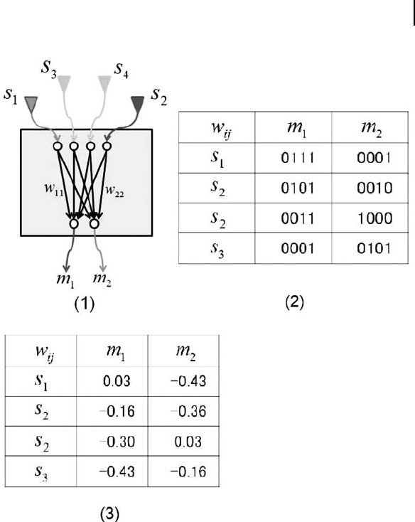
numerical sequence or character string (Fig. 7.14(1)). The machine
system as a phenotype may be a hexapod centipede or a function
unit that generates adequate output patterns in response to input
patterns.
In the discussion to follow, we consider the function unit of
Braitenberg’s robot shown in Fig. 7.12(1). The component with the
question mark (?) in the figure is the function unit.
Our robot has four sensors S
1
, S
2
, S
3
,andS
4
. When an external
stimulus is given to the sensors, the function unit responds and
outputs signals to two drive motors m
1
and m
2
. The behavior
expected for the robot is to “continue moving without collision as
much as possible.” We assume that the function unit incorporates
a single-layer neural network of four inputs and two outputs
(Fig. 7.14(1)). The structure of the network itself could be the result
of evolution, but we select a simple scenario for now.
We then determine genotypes and use four-digit binary se-
quences because of the ease of representation in genes. Since our
robot changes its behavior according to the synaptic weight, we
relate the genotype to the synaptic weight. We further assign values
to respective synaptic weights, which are the elements of the genes
in our example. The values are determined by generating random
numbers. The synaptic weights are four-digit binary numbers, which
are equivalent to 0 through 15 in the decimal system.
In our present study, we determine the synaptic weights as
follows:
(
w
11
, w
12
, w
21
, w
22
, w
31
, w
32
, w
41
, w
42
)
= (7, 1, 5, 2, 3, 8, 1, 5)
June 12, 2012 18:12 PSP Book - 9in x 6in 07-Junichi-Takeno-c07
Theory of Robot Evolution 119
Figure 7.14. Genotype and phenotype of a machine.
The function unit has eight synapses, each having a four-digit
synaptic value, i.e., the total number of bits of the genes of the
function unit is 32 (8 × 4). The respective synaptic values are
therefore represented in four bits as follows (Fig. 7.14 (2)):
w
ij
= (0111 0001 0101 0010 0011 1000 0001 0101)
The genes of this function unit are now finally determined as follows:
g = (01110001010100100011100000010101) (7.14)
This is the genotype of our robot. Let us now calculate the
phenotype for this genotype. Each synaptic value is divided by 15,
June 12, 2012 18:12 PSP Book - 9in x 6in 07-Junichi-Takeno-c07
120 Artificial Neural Networks and Machine Evolution
and 0.5 is subtracted from the result. This gives you the phenotype
(Fig. 7.14(3)). We divide by 15 to convert the synaptic values of
0 to 15 to values between 0 and 1.0. We subtract 0.5 to further
convert the resultant values to those between –0.5 and 0.5. Negative
numbers are intentionally introduced because inhibition values
must be considered for certain synaptic junctions.
We have thus converted the synaptic values to values suitable
for use in neural networks. It is assumed in our example that the
input and output values are real numbers, including negatives, and
therefore we use the values of the sigmoid function (x)towhich
0.5 is added as the threshold function of the neuro unit. This is
necessary, for example, to run the drive motors in reverse. Merits
include the fact that the sigmoid function is effective for inputs
between –1.0 and 1.0, and that values near zero are suitable for the
initial value of genes (Fig. 7.5 (1)).
It is somewhat difficult to understand that Fig. 7.14 (3) shows
the phenotype. The elements in the phenotype directly indicate
the synaptic values of the single-layer neural network built in the
function unit, and the actual robot (Fig. 7.14 (1)) behaves on the
basis of these synaptic values. As the phenotype is decided, the
robot’s behavior is also decided.
An explanation of population now follows. The genotype defined
by Eq. 7.14 is an initial value. Let us prepare, in our example, 20
genotypes as the initial value. Random numbers may be used. When
considering these 20 genotypes to be phenotypes, each behaves
differently. These 20 genotypes are therefore phenotypes of 20
individuals at the same time. These 20 individuals constitute the
population of the first generation.
Now we proceed to the selection process. We select individuals
with a high fitness function from among these 20 individuals. In our
example, robots capable of avoiding collision as much as possible are
determined to have a high fitness function. One possible evaluation
method would be to have each individual robot run and count the
number of collisions observed within a unit time. Assume we select
10 individuals.
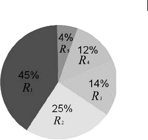
Various methods are available to select 10 individuals. One of
the popular methods is roulette wheel sampling. Individuals are
June 12, 2012 18:12 PSP Book - 9in x 6in 07-Junichi-Takeno-c07
Theory of Robot Evolution 121
Figure 7.15. Roulette wheel sampling.
selected by probability R
i
corresponding to relative fitness within
the given population (Fig. 7.15).
The widths of the regions on the roulette wheel are proportional
to the level of fitness. We spin the roulette wheel. When the pointer
stops at region R
3
, for example, the individual with that relevant
fitness is selected. If there is more than one individual, we select one
at random. Repeat this procedure 10 times, and you have selected
10 individuals. The advantage of the roulette wheel sampling is
that individuals with various levels of fitness are selected with a
certain balance for the given generation. “Balance” here means that
individuals of not only a high fitness but also those of a middle and
low fitness are selected as well. This method helps us approach the
optimum solution, or, in technical terms, avoids jumping at the local
maximum.
Assume the solution space for the distribution of genotype
solutions is as shown in Fig. 7.16.
The solution distribution in our example has two different
modes, each with a peak. This is a type of multimodal solution
distribution. Peak p
1
has a low fitness value compared with the
..................Content has been hidden....................
You can't read the all page of ebook, please click here login for view all page.