
Counters
Abstract
One of the most commonly used applications of flip-flops in practical systems is counters. They are used in microprocessors to count the program instructions (program counter or PC), for accessing sequential addresses in memory (such as ROM) or for checking progress of a test. Counters can start at any value, although most often they start at zero and they can increment or decrement. Counters may also change values by more than one at a time, or in different sequences (such as grey code, binary or binary coded decimal (BCD) counters).
24.1 Introduction
One of the most commonly used applications of flip-flops in practical systems is counters. They are used in microprocessors to count the program instructions (program counter or PC), for accessing sequential addresses in memory (such as ROM) or for checking progress of a test. Counters can start at any value, although most often they start at zero and they can increment or decrement. Counters may also change values by more than one at a time, or in different sequences, such as grey code, binary, or binary coded decimal (BCD) counters.
24.2 Basic Binary Counter using VHDL
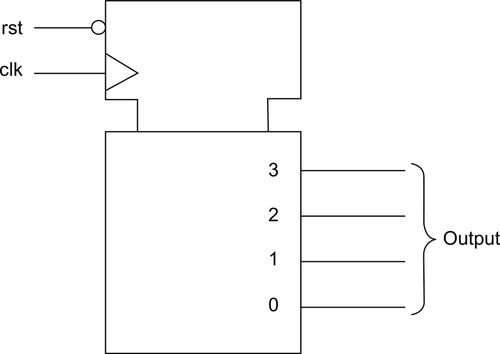
The simplest counter to implement in many cases is the basic binary counter. The basic structure of a counter is a series of flip-flops (a register), that is controlled by a reset (to reset the counter to zero literally) and a clock signal used to increment the counter. The final signal is the counter output, the size of which is determined by the generic parameter n, which defines the size of the counter. The symbol for the counter is given in Figure 24.1. Notice that the reset is active low and the counter and reset inputs are given in a separate block of the symbol as defined in the IEEE standard format.
From an FPGA implementation point of view, the value of generic n also defines the number of D type flip-flops required (usually a single LUT) and hence the usage of the resources in the FPGA. A simple implementation of such a counter is given here:
The important aspect of this approach to the counter VHDL is that this is effectively a state machine; however, we do not have to explicitly define the next state logic, as this will be taken care of by the synthesis software. This counter can now be tested using a simple test bench that resets the counter and then clocks the state machine until the counter flips round to the next counter round. The test bench is given as follows:
Using this simple VHDL test bench, we reset the counter until 2.5 μs and then the counter will count on the rising edge of the clock after 2 μs (i.e., the counter is running at 500 kHz).
If we dissect this model, there are several interesting features to notice. The first is that we need to define an internal variable count rather than simply increment the output variable q. The output variable q has been defined as a standard logic vector (std_logic_vector) and with it being defined as an output we cannot use it as the input variable to an equation. Therefore we need to define a local variable (in this case, count) to store the current value of the counter.
The initial decision to make is whether to use a variable or a signal. In this case, we need an internal variable that we can effectively treat as a sequential signal, and also one that changes instantaneously, which immediately requires the use of a variable. If we chose a signal, then the changes would only take place when the cycle is resolved (i.e., the next time the process is activated).
The second decision is what type of unit to use for the count variable. The output variable is a std_logic_vector type, which has the advantage of being an array of std_logic signals, and so we don’t need to specify the individual bits on a word; this is done automatically. The major disadvantage, however, is that the std_logic_vector does not support simple arithmetic operations, such as addition, directly. In this example, we want the counter to have a simple definition in VHDL and so the best compromise type that has the bitwise definition and also the arithmetic functionality would be the unsigned or signed type. In this case, we wish to have a direct mapping between the std_logic_vector bits and the counter bits, so the unsigned type is appropriate. Thus the declaration of the internal counter variable count is as follows:
The final stage of the model is to assign the internal value of the count variable to the external std_logic_vector q. Luckily, the translation from unsigned to std_logic_vector is fairly direct, using the standard casting technique:
As the basic types of both q and count are consistent, this can be done directly. The resulting model simply counts up the binary values on the clock edge as specified, as is shown in Figure 24.2.

24.3 Simple Binary Counter using Verilog
With the same basic specification as the VHDL counter, it is possible to implement a basic counter in Verilog using the same architecture of the model.
The model has the same connection points and operation, and will be treated in the same way for synthesis by the design software. The test bench is slightly different from the VHDL one in that it is much more explicit about the test function as well as the functionality of the test bench. For example, if we look at the top of the test bench Verilog has the $display and $monitor commands, which enable the time and variable values to be displayed in the monitor of the simulation as well as looking at the waveforms.
Using this test bench and Verilog model the behavior of the simulation can also be verified as shown in Figure 24.3.

24.4 Synthesized Simple Binary Counter
At this point it is useful to consider what happens when we synthesize this VHDL, so to test this point the VHDL model of the simple binary counter was run through a typical RTL synthesis software package (Leonardo Spectrum) with the resultant synthesized VHDL model given here:
The first obvious aspect of the model is that it is much longer than the simple RTL VHDL created originally. The next stage logic is now in evidence; as this is synthesized, the physical gates must be defined for the model. Finally the outputs are buffered, which leads to even more gates in the final model. If the optimization report is observed, the overall statistics of the resource usage of the FPGA can be examined (in this case, a Xilinx Virtex-II Pro device):
In this simple example, it can be seen that the overall utilization of the FPGA is minimal, with the relative resource allocation of IOs, buffers and functional blocks. This is an important aspect of FPGA design in that, even though the overall device may be underutilized, a particular resource (such as IO) might be used up. The output VHDL can then be used in a physical place and route software tool (such as the Xilinx Design Navigator) to produce the final bit file that will be downloaded to the device.
24.5 Shift Register
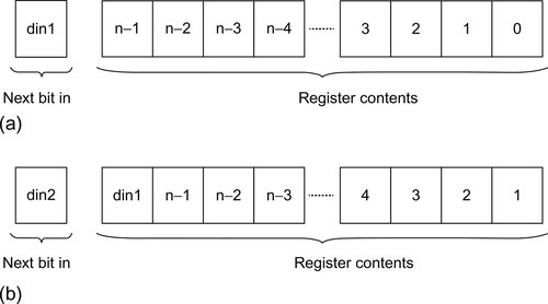
While a shift register is, strictly speaking, not a counter, it is useful to consider this in the context of other counters as it can be converted into a counter with very small changes. We will consider this element layer in this book, in more detail, but consider a simple case of a shift register that takes a single bit and stores in the least significant bit of a register and shifts each bit up one bit on the occurrence of a clock edge. If we consider an n-bit register and show the status before and after a clock edge, then the functionality of the shift register becomes clear, as shown in Figure 24.4.
A basic shift register can be implemented in VHDL as shown here:
The interesting parts of this model are very similar to the simple binary counter, but subtly different. As for the counter, we have defined an internal variable (shift_reg), but unlike the counter we do not need to carry out arithmetic functions, so we do not need to define this as an unsigned variable. Instead, we can define directly as a std_logic_vector, the same as the output q.
Notice that we have an asynchronous clock in this case. As we have discussed previously in this book, there are techniques for completely synchronous sets or resets, and these can be used if required.
The fundamental difference between the counter and the shift register is in how we move the bits around. In the counter we use arithmetic to add one to the internal counter variable (count). In this case, we just require shifting the register up by one bit, and to achieve this we simply assign the lowest (n − 1) bits of the internal register variable (shift_reg) to the upper (n − 1) bits and concatenate the input bit (din), effectively setting the lowest bit of the register to the input signal (din). This can be accomplished using the VHDL following:
The final stage of the model is similar to the basic counter in that we then assign the output signal to the value of the internal variable (shift_reg) using a standard signal assignment. In the shift register, we do not need to cast the type as both the internal and signal variable types are std_logic_vector:
We can also implement the shift register in Verilog, with the listing as shown here:
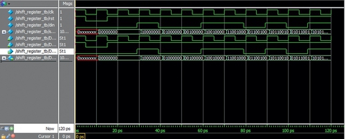
In both cases (VHDL and Verilog) we can test the behavior of the shift register by applying a data sequence and observing the shift register variable in the model, and in the case of the Verilog we can also add a $monitor command to display the transitions as they happen in the transcript of the simulator. The Verilog test bench code is given as:
The resulting simulation of the shift register can be seen in Figure 24.5.
24.6 The Johnson Counter
The Johnson counter is a counter that is a simple extension of the shift register. The only difference between the two is that the Johnson counter has its least significant bit inverted and fed back into the most significant bit of the register. In contrast to the classical binary counter with 2n states, the Johnson counter has 2n states. While this has some specific advantages, a disadvantage is that the Johnson counter has what is called a parasitic counter in the design. In other words, while the 2n counter is operating, there is another state machine that also operates concurrently with the Johnson counter using the unused states of the binary counter. A potential problem with this counter is that if, due to an error, noise or other glitch, the counter enters a state NOT in the standard Johnson counting sequence, it cannot return to the correct Johnson counter without a reset function. The normal Johnson counter sequence is shown in the following table:
The VHDL implementation of a simple Johnson counter can then be made by modifying the next stage logic of the internal shift_register function as shown in the following listing:
Notice that the concatenation is now putting the inverse (NOT) of the least significant bit of the internal state variable (j_state(0)) onto the next state most significant bit, and then shifting the current state down by one bit.
It is also worth noting that the counter does not have any checking for the case of an incorrect state. It would be sensible in a practical design to perhaps include a check for an invalid state and then reset the counter in the event of that occurrence. The worst-case scenario would be that the counter would be incorrect for a further 7 clock cycles before correctly resuming the Johnson counter sequence.
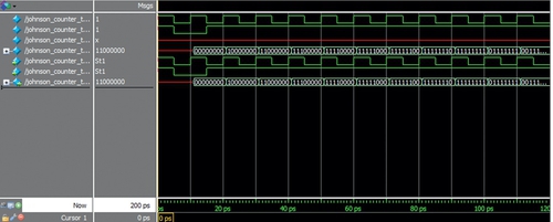
In a similar manner we can implement a Johnson counter in Verilog using the code given here:
and test it using the same basic counter test bench created for the simple counter, giving the simulation results as shown in Figure 24.6. We can see that the counter variable “ripples” through till it gets to all 1s and then carries back on until it is all 0s.
24.7 BCD Counter
The BCD (Binary Coded Decimal) counter is simply a counter that resets when the decimal value 10 is reached instead of the normal 15 for a 4-bit binary counter. This counter is often used for decimal displays and other human interface hardware. The VHDL for a BCD counter is very similar to that of a basic binary counter except that the maximum value is 10 (hexadecimal A) instead of 15 (hexadecimal F). The VHDL for a simple BCD counter is given in the following listing. The only change is that the counter has an extra check to reset when the value of the count variable is greater than 9 (the counter range is 0 to 9).
In a similar manner we can implement a BCD counter in Verilog using the code given here:
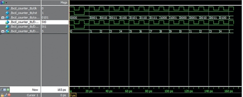
and test it using the same basic counter test bench created for the simple counter, giving the simulation results as shown in Figure 24.7. In the results this time you can see the counter variable in binary and also in unsigned decimal counting up to 1001 (binary) and 9 (decimal), then returning back to 0, giving the decimal counter.
24.8 Summary
In this chapter, we have investigated some basic counters and shown how VHDL and Verilog can be used to carry out arithmetic functions or logic functions to obtain the required counting sequence. The possibilities of counters based on these basic types are numerous, possibly infinite, and it is left to the readers to develop their own variations based on these standard types.
A useful exercise would be to modify the basic binary counter by adding an up/down flag so that, depending on this flag, the counter would increment or decrement respectively. Other options would be to extend the shift register to shift left or right depending on a directional flag.