Chapter 3. The Mini Toolbar and Other U.I. Improvements

In this chapter

Using the Mini Toolbar to Format Selected Text 54

Expanding the Formula Bar 58

Zooming In and Out on a Worksheet 59

Using the Status Bar to Add Numbers 60

Switching Between Normal View, Page Break Preview, and Page Layout View Modes 61

Using the New Sheet Icon to Add Worksheets 63

Although the ribbon and Quick Access toolbar are likely to be the most talked-about features in the new Excel interface, several other features are worth mentioning:

• Mini toolbar—The mini toolbar appears whenever you select text. Although this may happen rarely when you’re editing cells in Excel, it does happen frequently when you are working with charts, text boxes, and so on. The Mini toolbar offers quick access to font, size, bold, italics, alignment, color, indenting, and bullets.
• Formula bar—The formula bar includes the ability to expand or contract itself at your whim instead of the whim of Excel.
• Zoom slider—The Zoom slider allows you to quickly change from seeing one page to hundreds of pages at a time.
• Status bar—The status bar appears at the bottom of your worksheet window. Although you probably never noticed it, the status bar in previous versions of Excel reported the total of any selected cells. This information is now improved and expanded in Excel 2007.
• View control—The View control gives you one-click access to Page Break Preview mode, Normal mode, and the new Page Layout view.
• New Sheet icon—The New Sheet icon allows you to add new worksheets to a workbook with a single click.

Using the Mini Toolbar to Format Selected Text

The Mini toolbar is a shy attendant. When you select some text, almost imperceptibly, the Mini toolbar faintly appears above the text.

If you ignore the Mini toolbar, it fades away. However, if you move the mouse toward the Mini toolbar, the toolbar solidifies and offers you several text formatting options.

In your initial use of Excel 2007, you might not see the Mini toolbar. Although you often select cells or ranges of cells, it is rare to select only a portion of a cell value in Cell Edit mode.

However, as you begin using charts, SmartArt diagrams, and text boxes, you will have the Mini toolbar appearing frequently.

To use the Mini toolbar, you follow these steps:

1. Select some text. If you are selecting text in a cell, you must select a portion of the text in the cell by using Cell Edit mode. In a chart, SmartArt diagram, or text box, you can select any text.

   The Mini toolbar appears faintly. On some computers and with some color schemes, “faintly” actually means “completely transparently.”

2. Move the mouse pointer toward the Mini toolbar, and the toolbar solidifies. The Mini toolbar stays visible if your mouse is above it. After a period of inactivity, it disappears. If you move the mouse away from the Mini toolbar, it fades away.
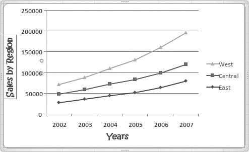
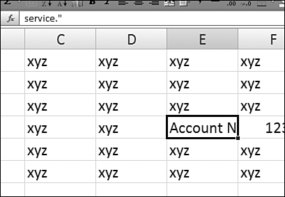
3. Make changes in the Mini toolbar to affect the text you selected in step 1. The Mini toolbar always has the same icons, even though some of them may not apply in the current situation. In Figure 3.1, for example, it does not make sense to apply indenting to the chart axis title, but the icons are always there and in the same place.

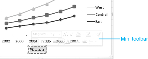
   Figure 3.1. You can barely make out the word Magneto above the number 2005. This is the Mini toolbar beginning to appear.

   

4. When you are done formatting the selected text, you can either move the mouse away from the Mini toolbar or use the Format Painter icon to apply the changes to additional text.
5. To use the Format Painter icon, click the paintbrush in the upper-right corner of the Mini toolbar. Then move toward other text in the document. The mouse pointer is a black-and-white paintbrush, to indicate that you are in Format Painter mode. When you click the other text, Excel applies the same formatting to the new text.

Initially, it is difficult to see the Mini toolbar. In Figure 3.1, look for the word Magneto just above the year 2005 on the x-axis. This word is the font name drop-down in the Mini toolbar. Plus, this is the second level of visibility; you actually have to have started moving your mouse toward the Mini toolbar in order to get it to appear this much.

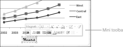
If you continue moving the mouse toward the Mini toolbar, it solidifies a bit more. In Figure 3.2, the mouse pointer is just outside the border of the Mini toolbar. At this point, you can start to identify all the controls on it.

Figure 3.2. As you move the mouse closer to the Mini toolbar, it begins to solidify.

In Figure 3.3, the Mini toolbar is completely visible. At this point, you can use any of its 14 controls in order to format the selected text.

Figure 3.3. In the fully visible state, the Mini toolbar offers a dozen controls for formatting text.

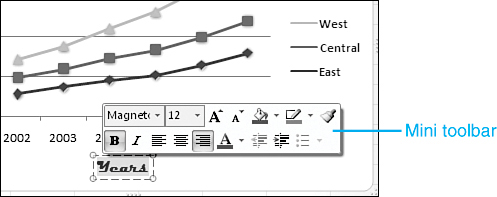
In the top row, the Mini toolbar offers five controls:

• Font name drop-down—You open this drop-down to choose a typeface. Each of the various font names is displayed in its own font so that you can select an appropriate font easily.
• Font Size drop-down—This drop-down offers font sizes from 8 to 96, in several increments.
• Increase Font Size icon—You click this icon to bump the font up to the next larger size.
• Decrease Font Size icon—You click this icon to make the font one size smaller.
• Format Painter—The format painter allows you to copy formatting from one place to another. (The format painter is discussed in detail in the following section.)

In the bottom row, the Mini toolbar offers nine controls:

• Bold icon—You use this to toggle bold on and off. If bold is already applied, the Bold icon has a glow effect around it.
• Italics icon—You use this to toggle italics on and off.
• Align Left icon—You click this control to left-align the text.
• Center Align icon—You click this control to center the text.
• Right Align icon—You click this control to right-align the text.
• Font Color drop-down—You use this drop-down to select a color. A menu item at the bottom of this drop-down allows you to display the Colors dialog box.
• Decrease Indent icon—You click this control to decrease the indent.
• Increase Indent icon—You click this control to increase the indent.
• Bullet drop-down—You can choose from seven styles of bullets or none. A menu item at the bottom of the drop-down allows you to open the Bullets and Numbering dialog box.

Using the Format Painter to Copy Formats

After you have formatted the selected text by using the Mini toolbar, you might want to apply the same formatting to other text. To do so, you follow these steps:

1. Click the Format Painter icon in the upper-right corner of the Mini toolbar.
2. Move your mouse away from the Mini toolbar, and it disappears. Your mouse pointer is now in the shape of a paintbrush, as shown in Figure 3.4.

   Figure 3.4. The paintbrush icon indicates that the selected format will be applied to whatever you select next.

   

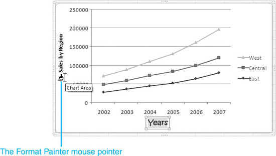
3. Click the vertical axis title. The selected format is applied, as shown in Figure 3.5.

Figure 3.5. You can click another text element to apply the same formatting you have applied to other text.

Getting the Mini Toolbar Back

The shyness of the Mini toolbar might be the most frustrating part of using it. If you move the mouse away from the Mini toolbar, it fades away. If you immediately move back toward the Mini toolbar, it comes back. If you use the mouse for some other task, such as scrolling, the Mini toolbar permanently goes away. In this case, you might have to re-select the text in order to get the Mini toolbar to come back.

Disabling the Mini Toolbar

If you are annoyed by the Mini toolbar, you can turn it off for all Excel workbooks. Here’s what you do:

1. Select Office Icon, Excel Options.
2. In the Personalize category of the Excel Options dialog, clear the Show Mini Toolbar on Selection check box.

Expanding the Formula Bar

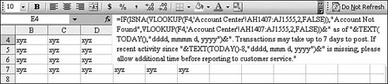
Formulas range from very simple to the very complex. As people began writing longer and longer formulas in Excel, an annoying problem began to appear: If the formula for a selected cell was longer than the formula bar, the formula bar would wrap and extend over the worksheet (see Figure 3.6). In many cases, the formula would obscure the first few rows of the worksheet. This was frustrating, especially if the selected cell was in the top few rows of the spreadsheet.

Figure 3.6. In prior versions of Excel, the formula bar could obscure cells on a worksheet. In this case, both the active cell, E4, and the dependent cell, F4, are hidden.

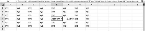
Excel 2007 features a new formula bar that prevents the formula from obscuring the spreadsheet. For example, in Figure 3.7, Cell E4 contains a formula that is longer than the formula bar. Notice the two new controls at the right end of the formula bar: a scrollbar and Expand Formula Bar icon (which looks like a down-pointing double arrow).

Figure 3.7. By default, Excel 2007 shows the initial portion of the formula.

You use the formula bar scrollbar to scroll through the formula, one line at a time. You use the Expand Formula Bar icon to expand the formula bar. As shown in Figure 3.8, expanding the formula bar actually moves the grid down. This way, you can see the formula bar and still see the cells in the grid, too. In expanded mode, the Expand Formula Bar icon is replaced by a double up-pointing arrow that you can use to contract the formula bar back to one line.

Figure 3.8. You can click a button to expand the formula bar.

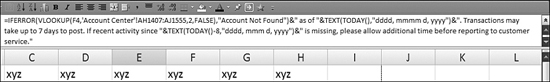
After you collapse the formula bar, Excel has the annoying tendency to show only the last line of the formula. This could be confusing, especially if you look in the formula bar to learn whether a cell starts with an equals sign. For example, someone new to the spreadsheet shown in Figure 3.9 might not understand that Cell E4 contains a formula.

Figure 3.9. After you collapse the formula bar, it might show only the last line of the formula. This is a confusing view because it is not obvious how the cell value can result from this formula bar.

Zooming In and Out on a Worksheet

In the lower-right corner of the Excel window, a new Zoom slider allows you to zoom from 400% to 10% with lightning speed. You simply drag the slider to the right to zoom in and to the left to zoom out. The Zoom Out and Zoom In buttons on either end of the slider allow you to adjust the zoom in 10% increments.

Figure 3.10 shows the zoom control set to the maximum zoom of 400%.

Figure 3.10. You can use the Zoom slider or the Zoom Out and Zoom In buttons to change the zoom.

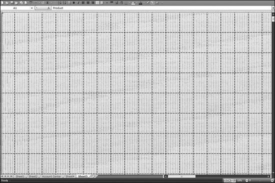
At the opposite end of the zoom spectrum, the 10% view shows an overview of 158 printed pages of the worksheet. As shown in Figure 3.11, you cannot make out any numbers at a 10% zoom. However, in the 40%–60% zoom range, you can see 3 to 10 pages and actually make out the numbers in the cells.

Figure 3.11. At 10% zoom, you can see 150+ pages at once.

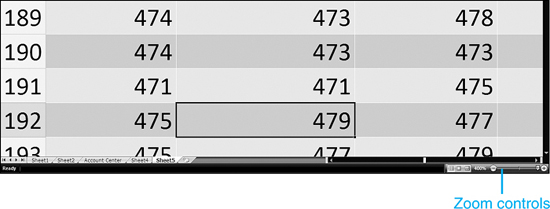
Using the Status Bar to Add Numbers

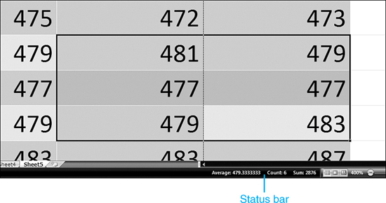
If you select several cells that contain numeric data and then look at the status bar, at the bottom of the Excel window, you can see that the status bar reports the average, count, and sum of the selected cells (see Figure 3.12).

Figure 3.12. The status bar shows the sum, average, and count of the selected cells.

If you need to quickly add the contents of several cells, you can simply select the cells and look for the total in the status bar. This feature has been in Excel for a decade, yet very few people realized it was there. In prior versions of Excel, only the sum would appear, but you could right-click the sum in order to see other values, such as the average, count, minimum, and maximum.

As with past versions of Excel, in Excel 2007 you can customize which statistics are shown in the status bar. In Excel 2007, you can configure all of the status bar elements. To do so, you right-click the status bar to display the Status Bar Configuration panel. In this panel, you can see the current value of all status bar icons, whether they are hidden or not (see Figure 3.13).

Figure 3.13. You can configure the status bar to show or hide all these indicators.

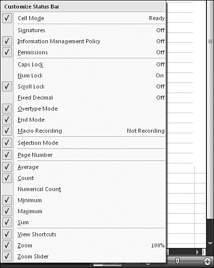
To add new items to the status bar, you click them in the Status Bar Configuration panel.

Switching Between Normal View, Page Break Preview, and Page Layout View Modes

Three shortcut icons in the status bar allow you to quickly switch between three view modes as shown in Figure 3.14:

Figure 3.14. Three view shortcuts appear in the status bar.

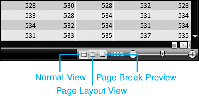
• Normal View—This mode shows worksheet cells as normal.
• Page Break Preview—This mode draws the page breaks with blue. You can actually drag the page breaks to new locations in Page Break preview. This mode has been available in several versions of Excel.
• Page Layout View—This is a new view in Excel 2007. It combines the best of Page Break Preview and Print Preview modes.

In Page Layout View mode, each page is shown, along with the margins, header, and footer. A ruler appears above the pages and to the left of the pages. You can make changes in this mode in the following ways:

• To change the margins, you drag the gray boxes in the ruler.
• To change column widths, you drag the borders of the column headers.
• To add a header, you click Click to Add Header.

Figure 3.15. The new Page Layout View mode gives a view of page breaks, margins, headers, and footers.

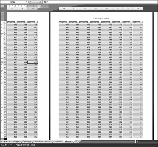
Because it is possible to navigate and enter formulas in any of the view modes, you might want to do actual worksheet editing in the new Page Layout View mode.

Using the New Sheet Icon to Add Worksheets

The final new control in the Excel 2007 user interface is the Insert Worksheet icon. This icon appears as a small worksheet tab with a New icon. The tab appears to the right of the last worksheet tab, as shown in Figure 3.16.

Figure 3.16. Add a new worksheet to the end of your workbook by using the New Worksheet icon.

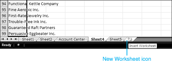
You click the icon to add a new worksheet to the end of the workbook.

Dragging a Worksheet to a New Location

After a worksheet has been added to the end of the workbook, you can drag the sheet to a new location in the middle of the workbook. Follow these steps to move a worksheet to a new location:

1. Click on the Worksheet tab.
2. Drag the mouse left or right. The mousepointer shows a sheet of paper under the mousepointer.
3. Watch for the insertion triangle just above the row of sheet names. In general, the insertion triangle will indicate that the sheet is dropped to the left of the sheet you are hovering above.
4. When the insertion triangle is in the correct location, release the mouse button.

The worksheet will be moved to the new location.

Inserting a Worksheet in the Middle of a Workbook

Although using the New Worksheet icon and then dragging a worksheet to a new location is easier, you can also insert a worksheet in a particular location. To insert a worksheet to the left of the current worksheet, for example, you choose Home, Cells, Insert, Insert Sheet. The new sheet is added before the current sheet.

Alternatively, you can right-click any sheet and choose Insert. The Insert dialog appears, where you can choose to insert a worksheet or a variety of templates. The new sheet appears to the left of the selected tab.