Chapter 32. Formatting Worksheets

In this chapter

Why Format Worksheets? 892

Using Traditional Formatting 893

Formatting with Styles 914

Other Formatting Techniques 915

Copying Formats 921

Formatting adds interest and readability to documents. If you have taken time to create a spreadsheet, you should also take the time to make sure that it is eye catching and readable.

You can format documents in Excel 2007 with any of these three methods:

• Use tables styles—As described in Chapter 8, “Fabulous Table Intelligence,” you can use table styles to quickly format a table with banded rows, accents for totals, and so on.
• Use cell styles—You can use cell styles to identify titles, headings, and accent cells. The advantage of using cell styles is that you can quickly apply new themes to change the look and feel of a document.
• Use formatting commands—You can use traditional formatting commands to change the font, borders, fill, numeric formatting, columns widths, and row heights. The usual formatting icons are now found on the Home ribbon as well as in the Format Cells dialog box.

Why Format Worksheets?

You could easily open a blank worksheet and fill it with data without ever touching any of Excel’s formatting commands. The result would be functional but not necessarily readable or eye catching.

Figure 32.1 contains an unformatted report in Excel.

Figure 32.1. After typing data into a spreadsheet, you have an unformatted report.

Figure 32.2 contains exactly the same data but with formatting applied. The formatted report is more interesting than the unformatted one. The reader can instantly focus on the totals for each line. Headings are aligned with the data. Borders break the data into sections. Accent colors highlight the subtotals and totals. The title is prominent, in a larger font and headline typeface. Numeric formatting has removed the extra decimal places and added thousands separators. The column widths are adjusted properly. A short row adds a visual break between the product lines. Headings for each product line are rotated, merged, and centered.

Figure 32.2. Readability is improved after formatting the report.

The formatting applied to Figure 32.2 takes a few extra minutes, but it dramatically increases the readability of the report. You’ve taken the time to put the worksheet together, and it is worth a couple minutes to help the consumer of the worksheet easily read it.

Using Traditional Formatting

Formatting is typically carried out in the Format Cells dialog box or using the formatting icons located on the Home ribbon.

In Excel 2007, Microsoft took the icons formerly on the Formatting toolbar and arranged them in the Font, Alignment, and Number groups on the Home ribbon, as shown in Figure 32.3. Additional column- and row-formatting commands are available in the Format drop-down in the Cells group on the Home ribbon.

Figure 32.3. Most icons from the former Formatting toolbar are in the Font, Alignment, and Number tabs on the Home ribbon.

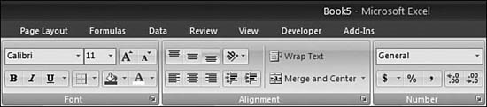
While analyzing SQM data from Microsoft Excel 2003, the Excel 2007 development team decided to promote some settings from the Format Cells dialog to the Home ribbon. Icons for wrapping text, vertical alignment, and text rotation have therefore been added to the icons formerly on the Formatting toolbar.

If your favorite setting is not on the Home ribbon, you can take one of the four entry paths to the Format Cells dialog, which provides access to additional settings, such as Shrink to Fit, Strikethrough, and more border settings:

• Press Ctrl+1 (that is Ctrl and the number 1). You can press Ctrl+Shift+F to display the Font tab on the same dialog.
• Click the double-diagonal arrow icons in the lower-right corner of the Font, Alignment, or Number groups. Each icon opens the dialog, with the focus on a different tab.
• Right-click any cell and choose Format Cells.
• On the Home ribbon, select Cells, Format, Format Cells.

As shown in Figure 32.4, the Format Cells dialog includes six tabs:

Figure 32.4. The Format Cells dialog offers complete control over cell formatting. You can visit this dialog when the icons on the ribbon don’t provide enough detail.

• Number—The Number tab gives you absolute control over numeric formatting. You can choose from 96,885 built-in formats or use the Custom category to create your own.
• Alignment—The Alignment tab offers settings for horizontal alignment, vertical alignment, rotation, wrap, merge, and shrinking to fit.
• Font—The Font tab controls font, size, style, underline, color, strikethrough, superscript, and subscript.
• Border—The Border tab controls line style and color for each of the four borders and the diagonals on each cell.
• Fill—The Fill tab offers 16 million fill colors, patterns, and now, for Excel 2007, cell gradients.
• Protection—You can use the Protection tab to lock or unlock certain cells. See Chapter 34, “Sharing Workbooks with Others,” for more information.

Changing Numeric Formats by Using the Home Ribbon

Do you ever go shopping for hardware at a general-purpose store? I am amazed at their ability to have almost what I need but to never actually have what I need. I usually end up cursing my decision to stop at the general-purpose retailer and drive another mile down the road to Home Depot or Lowe’s, where they always have exactly what I need.

Using the Number group on the Home ribbon is like shopping at a general-purpose retailer. It has a lot of settings for numeric formatting, but most of the time, they are not exactly what you need, and you end up visiting the Number tab on the Format Cells dialog.

To start, there are three icons, for currency, percentage, and comma style. The Percentage icon is useful. Unfortunately, the Currency and Comma icons both apply an Accounting style to a cell, and the Accounting style is inappropriate for everyone except accountants. Furthermore, these three icons are not toggle buttons. When you use one of them, there is not an icon to quickly go back to a general style (other than Undo).

The Increase and Decrease Decimal icons are useful. Each click of one of these buttons forces Excel to show one more or one fewer decimal place. If you have numbers showing two decimal places in all cells, a couple clicks on the Decrease Decimal icon solves the problem.

Figure 32.5 shows the Currency, Percentage, Comma, Increase Decimal, and Decrease Decimal buttons in the Number group of the Home ribbon.

Figure 32.5. The Currency and Comma icons both use an Accounting style. This is wonderful for accountants, but others should resist using them.

Above the five buttons in the Number group is a new drop-down that has a dozen popular number styles. Figure 32.6 shows the styles in the drop-down. The range A2:F12 shows these styles applied to four different numbers.

Figure 32.6. Excel 2007 offers 12 popular number styles in this drop-down.

Here are some comments and cautions about using the number styles from the drop-down in the Home ribbon:

• General Format is a number format. Decimal places are shown if needed. No thousands separator is used. A negative number is shown with a minus sign before the number.
• Number does not use a thousands separator. It forces two decimal places, even with numbers that don’t need decimal places, such as in Cell E3.
• Currency is a useful format for everyone. The currency symbol is shown immediately before the number. All numbers are expressed with two decimal places. Negatives are shown with a hyphen before the number.
• Accounting is great for financial statements and annoying for everything else. Negative numbers are shown in parentheses. Currency symbols are left-aligned with the edge of the cell. Positive numbers appear one character from the right edge of the cell to allow them to line up with negative numbers.
• Percentage uses two decimal places when selected from the drop-down. This is one format for which it is actually better to use the icon on the ribbon than the Format Cells dialog.
• Fraction defaults to showing a fraction with a one-digit divisor. If you have a number such as 0.925, some Excel number formats would correctly show this as 15/16. Unfortunately, the Fraction setting in this drop-down rounds it to 1.

Changing Numeric Formats by Using Built-in Formats in the Format Cells Dialog

The Format Cells dialog offers far more number formats than the Home ribbon. My favorite number format can only be accessed through the Format Cells dialog. I find that I avoid the buttons in the Number group in the Home ribbon and go directly to the Format Cells dialog.

You display the Format Cells dialog by clicking the double-diagonal arrow icon in the lower-right corner of the Number group of the Home ribbon. When you open the Format Cells dialog this way, the Number tab is the active tab.

There are 12 categories on the left side of the Number tab. The General and Text categories each have a single setting. The Custom category allows you to use formatting codes to build any number format. The remaining nine categories each offer a collection of controls to customize the numeric format.

Using Numeric Formatting with Thousands Separators

Using numeric formatting with thousands separators is my favorite format. The thousands of separators make the number easy to read. You can easily suppress the cents from the numbers. Microsoft does not offer buttons on the Home ribbon to select this format. The comma button would be a perfect place for it, but instead, Microsoft assigns that to the accounting format.

To format cells in numeric format, you follow these steps:

1. Press Ctrl+1 to display the Format Cells dialog.
2. Choose the Number category from the Number tab.
3. Check the box Use 1000 Separator.
4. Optionally, adjust the Decimal Places spin button to 0.
5. Optionally, select a method for displaying negative numbers.

Figure 32.7 shows the Number category of the Format Cells dialog.

Figure 32.7. The Number category is the workhorse in Excel.

Displaying Currency

There are two categories for currency. The Currency category is identical to the Number category shown in Figure 32.7, with the addition of a currency symbol drop-down. This drop-down offers 390 different currencies from around the world.

The second category, Accounting, always shows negative numbers in parentheses. With this category, the currency symbol is always left-aligned in the cell. The last digit of positive numbers appears one character from the right edge of the cell so that positive and negative numbers line up.

Displaying Dates and Times

The Date category offers 17 built-in formats for displaying dates. The Time category offers nine built-in formats for displaying time. Each category has two formats that display both date and time.

The date formats vary from short dates, such as 3/14, to long dates, such as Wednesday, March 14, 2001. You should pay particular attention to the Date formats and the Sample box. Some formats show only the month and the day. Other formats show the month and the year. The values in the Type box are for March 14, 2001. Types such as March-01 display month-year. Types such as 14-Mar are displaying day-month.

An interesting format near the bottom of the list is the M type. This displays month names in JFMAMJJASOND style, as shown in Figure 32.8. Readers of the Wall Street Journal’s financial charts will instantly recognize that in this style, each month is represented by the first letter of the month. It works great when used as the labels along the x-axis of a chart.

Figure 32.8. A variety of date and time formats are available.

In the Time category, you should pay attention to an important distinction between the 1:30 PM, 13:30, and 37:30:55 types. The first type displays times from 12:00 AM through 11:59 PM. The second type displays military time. In this system, midnight is 0:00, and 11:59 PM is 23:59. Neither of these types displays hours in excess of 24 hours. If you are working on a weekly timesheet or any application where you need to display hours that total to more than 24 hours, you need to use the 37:30:55 type in the Time category. This format is one of few that displays hours in excess of 24.

Displaying Fractions

The Fractions category rounds a decimal number to the nearest fraction. Types include fractions in halves, quarters, eighths, sixteenths, tenths, and hundredths. In addition, the first three types specify that the decimal should be reduced to the nearest fraction with up to one, two, or three digits in the denominator.

Figure 32.9 shows a variety of decimals formatted with five different fractional types. In Row 14, notice that this random number can appear as 1/2, 49/92, or 473/888 when using the Up To n Digit types. Excel rounds the number to the closest fraction.

Figure 32.9. Excel can display decimals as fractions in a variety of formats.

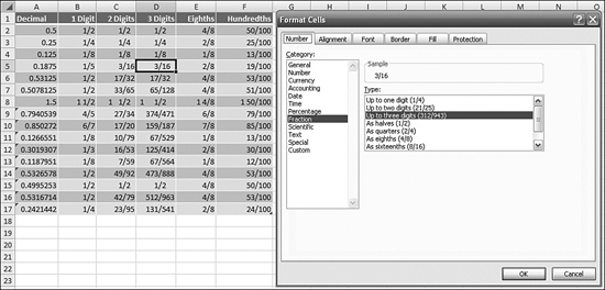
In Column E, note that if you ask Excel to show the number in eighths, Excel uses 4/8 and 2/8 instead of 1/2 or 1/4.

I am sure that I spent way too much time in junior high math learning how to reduce fractions. The first three fraction types of number formatting in Excel eliminate the need for manually reducing fractions.

Displaying Zip Codes, Telephone Numbers, and Social Security Numbers

Spreadsheets were invented in Cambridge, Massachusetts. If you enter the zip code for Cambridge (02138) in a cell, Excel does not display the zip code correctly. It truncates the leading zero, giving you a zip code of 2138.

To combat this problem, Excel provides four special formatting types, all of which are U.S. centric:

• The Zip Code and Zip Code + 4 styles ensure that east coast cities do not lose the leading zeros in their zip codes.
• The Phone Number type formats a telephone number with parentheses around the area code and a hyphen after the exchange.
• The Social Security Number type groups the digits into groups of three, two, and four numbers, separated by hyphens.

Figure 32.10 shows cells formatted with the four types, which are available in the Special category.

Figure 32.10. U.S. customers will appreciate the Special category in the Format Cells dialog.

Changing Numeric Formats Using Custom Formats

Custom number formats provide incredible power and flexibility. Although you don’t need to know the complete set of rules for them, you will probably find a couple custom number formats that work perfectly for you and be able to make use of them.

To use a custom number format, you follow these steps:

1. Select the cells to be highlighted.
2. Display the Format Cells dialog by pressing Ctrl+1
3. Choose the Number tab.
4. Choose the Custom category.
5. Type the formatting codes in the Type box. Excel shows you a sample of the active cell formatted with this format in the Sample box.
6. Make sure this format looks correct and then click OK to accept it.

Using the Four Zones of a Custom Number Format

A custom number format can contain up to four different formats, each separated by a semicolon. The semicolons divide the format into up to four zones. Excel allows different formatting, depending on whether a cell contains a positive number, negative number, zero, or text. You need to keep in mind the following:

• Separate formatting codes for zones by using semicolons.
• If you type only one number format, it applies to all numbers.
• If you type only two formats, the first format applies to positive and zero. The second format is used for negative.
• If all four formats are used, they refer to positive, negative, zero, and text values, respectively.

In Figure 32.11, a custom number format uses all four zones. The table in Rows 11:14 shows how various numbers are displayed in this format. (Cell B14 appears in red type.)

Figure 32.11. The four zones of a custom number format can cause positive, negative, zero, and text values to display differently.

Controlling Text and Spacing in a Custom Number Format

You can display a mix of text and numbers in a numeric cell. To do so, you simply include the text in double quotation marks. For example, "The total is "$#,##0 precedes the number with the text shown in quotes.

If you need a single character, you can omit the quotation marks and precede the character with a backslash (). For example, the code $#,##0,,M displays numbers in millions and adds an M indicator after the number.

Some characters require neither a backslash nor quotation marks. These special characters are $ - + / ( ) : ! & ' ~ { } = < > and the space character.

To add a specific amount of space to a format, you enter an underscore followed by a character. Excel then includes enough space to include that particular character. One frequent use for this is to include _) at the end of a positive number to leave enough space for a closing parenthesis. The positive numbers then line up with the negative numbers shown in parentheses.

To fill the space in a cell with a repeating character, you use an asterisk followed by the character. For example, the format **0 fills the leading space in a cell with asterisks. The format 0*- fills the trailing space in a cell with hyphens.

If you are expecting numbers but think you might occasionally have text in the cell, you can use the fourth zone of the format. You use the @ character to represent the text in the cell. For example, 0;0;0;"Unexpected entry of "@ highlights the text cells with a note.

Controlling Decimal Places in a Custom Number Format

You use a zero as a placeholder when you want to force the place to be included. For example, 0.000 formats all numbers with three decimal places. If the number has more than three places, it will be rounded to three decimal places.

You use a pound sign (#) as a placeholder to display significant digits but not insignificant zeros. For example, 0.### displays up to three decimal places, if needed, but can display 1. for a whole number.

You use a question mark to replace insignificant zeros on either size of the decimal point with enough space to represent a digit in a fixed-width font. This format was designed to allow decimal points to line up, but with proportional fonts, it may not always work.

To include a thousands separator, you include a comma to the left of the decimal point. For example, #,##0 displays a thousands separator.

To scale a number by thousands, you include a comma after the numeric portion of the format. Each comma divides the number by a thousand. For example, 0, displays numbers in thousands, and 0,, displays numbers in millions.

Using Conditions and Color in a Custom Number Format

The condition codes available in numeric formatting predate conditional formatting by a decade. You should consider the flexible conditional formatting features (see Chapter 9, “Visualizing Data in Excel”) for any new conditions, but in case you encounter an old worksheet with these codes, it is valid to use eight colors in the format: red, blue, green, yellow, cyan, black, white and magenta. You include the color in square brackets. It should be the first element of any numeric formatting zone.

You can include a condition in square brackets after the color but before the numeric formatting. For example, [Red][<=100];[Blue][>100] displays numbers under 100 in red and other numbers in blue. The U.S. telephone special format uses this custom condition [<=9999999]###-####;(###) ###-####.

Using Dates and Times in a Custom Number Format

Although many of these settings are arcane, I still regularly use many of the date and time formats shown in Table 32.1. The various m and d codes allow flexibility in expressing dates.

Table 32.1. Date and Time Formats

The custom number format m/d/yy displays the month and day numbers as one digit if possible. For example, dates formatted with this code would display as 1/9/08, 1/31/08, 9/9/09, and 12/31/08.

A custom number format of mm/dd/yy always uses two digits to display the month and day. Examples are 01/09/08 and 01/31/08.

The remaining date and time codes can display months as Jan, January, or J and days as 1, 01, Fri, or Friday.

Displaying Scientific Notation in Custom Number Formats

To display numbers in scientific format, you use E-, or E+ exponent codes in a zone.

If a format contains a zero (0) or pound sign (#) to the right of an exponent code, Excel displays the number in scientific format and inserts an E. The number of zeros or pound signs to the right of a code determines the number of digits in the exponent. E- or e- places a minus sign by negative exponents. E+ or e+ places a minus sign by negative exponents and a plus sign by positive exponents.

Take the following, for example:

• 1450 formatted with 0.00E+00 would display as 1.45E+03
• 1450 formatted with 0.00E-00 would display as 1.45E03
• 0.00145 formatted with either code would display 1.45E-03

Aligning Cells

Worksheets look best when the headings above a column are aligned with the data in the column. Excel’s default behavior is to left-align text and to right-align values and dates.

On the left side of Figure 32.12, the month headings in Row 5 are left-aligned, and the numeric values starting in Row 6 are right-aligned. This makes the worksheet look haphazard. To solve the problem, you can right-align the headings cells. The right side of Figure 32.12 shows the headings right-aligned.

Figure 32.12. In the left side of the image, the left-aligned headings appear out of alignment with the numbers. The worksheet on the right shows the headings after the Right Align icon is clicked.

To right-align cells, you select the cells and click the Right Align icon in the Alignment group of the Home ribbon.

Changing Font Size

There are three icons in the Font group of the Home ribbon for changing font size:

• The Increase Font Size (A^) icon increases the font size in the selected cells to the next larger setting.
• The Decrease Font Size (A^v) icon decreases the font size in the selected cells to the next smaller setting.
• The Font Size drop-down offers a complete list of font sizes. You can hover over any font size to see the Live Preview of that size in the selected cells of the worksheet (see Figure 32.13).

Figure 32.13. When you use the Font Size drop-down, Live Preview shows you the effect of an increased font before you select the font.

Changing Font Typeface

Changing the font typeface is vastly improved in Excel 2007. For a couple versions, the Font drop-down has been able to show the font names in the style of each font. Now, in Excel 2007, as you hover over the font, Live Preview shows you how the font will look in the selected cells in your worksheet, as shown in Figure 32.14. The Font name drop-down is in the Font group of the Home ribbon.

Figure 32.14. The Font drop-down in the Home ribbon now shows you the look of each font, and Live Preview shows you how your individual cells will look with the font applied.

Applying Bold, Italic, and Underline

Three icons in the Font group in the Home ribbon allow you to change the font to apply bold, italic, and underline. Unlike the icons in the Number group, these icons behave properly, toggling the property on and off. The Bold icon is a bold letter B. The Italic icon is an italic letter I. The Underline icon is either an underlined U or a double-underlined D. The Underline icon is actually a drop-down. As shown in Figure 32.15, you can choose the drop-down to change from Single Underline to Double Underline.

Figure 32.15. Bold, Italic, and Underline icons toggle the style on and off for the selected cells.

The underline style underlines the characters in the cell. If you have a cell that contains 123, the underline is 3 characters wide. If you have a cell with 1,234,567.89, the underline is 12 characters wide. If you need an underline to extend the entire width of a cell, you can select Single Accounting Underline or Double Accounting Underline on the Font tab of the Format Cells dialog. Or you can use a bottom border in the cell.

Using Borders

There are 1.7 billion unique combinations of borders for any four-cell range. The Borders drop-down in the Font group of the Home ribbon offers 13 of the most popular options, as shown in Figure 32.16.

Figure 32.16. The Borders drop-down offers 13 of the most popular border choices.

To apply borders to a range, you follow these steps:

1. Select the range.
2. On the Home ribbon, in the Font group, open the Borders drop-down.
3. Select one of the 13 presets from the drop-down. Live Preview does not work with borders, so you have to select a border before you see the effects.
4. If the presets do not present the combination you need, select More Borders from the drop-down to display the Borders tab of the Format Cells dialog.
5. In the Format Cells dialog, choose a line style from the Line section of the Borders tab.
6. Choose a color from the Color drop-down.
7. Draw borders by using one of the 11 preset buttons in the drop-down or click in and around the Text Text Text Text box.
8. If you need to mix colors in the range (for example, a blue top border and a red bottom border), repeat steps 5 through 7 for the other color or line style.
9. Click OK to apply the border.

There is an important concept to understand when applying borders to a range. Say that you select 20 rows by 20 columns (for example, cells A1:T20). If you apply a top border by using the drop-down, only the top row of cells A1:T1 have the border. Often, this is not what you were expecting. You might have wanted a border on the top of all 400 cells. In the Format Cells dialog box, there is a representation of a 2×2 cell range, as shown in Figure 32.17. The border style drawn in the top edge of this box affects only the top edge of the range. The border style drawn in the middle horizontal line of the box affects all the horizontal borders on the inside of the selected range.

Figure 32.17. If you need to change the color or the line style of the borders, you use the Format Cells dialog.

The fastest way to select all horizontal and vertical borders in the range is to click the Outline button and then the Inside button in the Presets section of the dialog.

Coloring Cells

Excel 2007 adds the ability to use a gradient to fill a cell. This can provide an interesting look for a title cell. Gradient formatting is available only in the Format Cells dialog.

The Font group on the Home ribbon offers a paint bucket drop-down and an A drop-down. The paint bucket is a color chooser for the background fill of the cell. The A drop-down is a color chooser for the font color in the cell. Both drop-downs offer 6 shades of the 10 theme colors, 10 standard colors, and the option More Colors. The paint bucket drop-down also offers the menu choice No Fill, as shown in Figure 32.18.

Figure 32.18. The color drop-down offers theme colors, 10 standard colors, and the link More Colors.

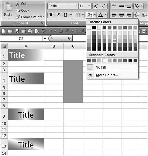
The More Colors drop-down offers the two-tabbed Colors dialog. You can either choose a color from the Standard tab or enter an RGB value on the Custom tab.

The two-color gradient in a cell is a new feature in Excel 2007. To activate this feature, you follow these steps:

1. Select one or more cells. If you select a range of cells, Excel repeats the gradient for each cell in the range.
2. Press Ctrl+1 to display the Format Cells dialog.
3. Choose the Fill tab.
4. Click the Fill Effects button.
5. In the Color 1 and Color 2 drop-downs, choose two colors or choose one color and white.
6. In the Shading Styles section, choose a shading style.
7. In the Variants section, choose one of the three variations. A sample is shown in the Sample box.
8. Click OK to close the Fill Effects dialog.
9. Click OK to close the Format Cells dialog.

Figure 32.19 shows the Fill Effects dialog. Cell A1 contains a vertical shading, from left to right. Cell A4 shows the opposite variant of vertical shading. Cell A9 shows the from-the-center variant of the vertical shading. Cell A13 shows a diagonal-down shading style.

Figure 32.19. In Excel 2007, you can add gradients as the fill within cells.

Adjusting Column Widths and Row Heights

You can adjust the width of every column in a worksheet. In many cases, narrowing the columns to reduce wasted space can allow a report to fit on one page.

I always say that there are three or more ways to accomplish most tasks in Excel. In most cases, I have a favorite method to do any task and use that method exclusively. However, setting column widths and row heights is a task where I actively use many different methods, depending on the circumstances.

You can use the following seven methods to adjust column width. Every one of them applies equally well to adjusting row heights:

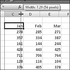
• Click the border between the column headings—As shown in Figure 32.20, you can drag to the left to make the column narrow. You can drag to the right to make the column wide. A ToolTip appears, showing the width in points and pixels. The advantage of this method is that you can simply drag until the column feels like it is the right width. The disadvantage is that this method fixes one column at a time.

Figure 32.20. The right border between one cell letter and the next is the key to adjusting column widths.

• Double-click the border between column headings—Excel automatically adjusts the left column to fit the widest value in the column. The advantage of this method is that the column is exactly wide enough for the contents. The disadvantage is that a very long title in Cell A1 makes this method ineffective. You might have been planning on allowing the title in Cell A1 to spill over to B1, C1, and D1. However, the double-click method makes the column wide enough for the long title. (In this case, you want to use the final method in this list.)
• Select many columns and drag the border for one column—When you do this, the width for all columns is adjusted. The advantage of this method is that you can adjust all columns at once, and they are all a uniform width.
• Select many columns and double-click one of the borders between column letters—When you do this, all the columns adjust to fit their widest value.
• Use the ribbon—Select one or more columns. From the Cells group of the Home ribbon, select Format, Column Width. Then you enter a width in characters and click OK.
• Apply one column’s width to other columns—If there is one column that is a suitable width, and you want all other columns to be the same width, you should use this method. You select the column with the correct width. Then you press Ctrl+C to copy. Next, you select the columns to be adjusted. Next, you choose the Clipboard section of the Home ribbon and select Paste, Paste Special, Column Widths. Finally, you click OK.
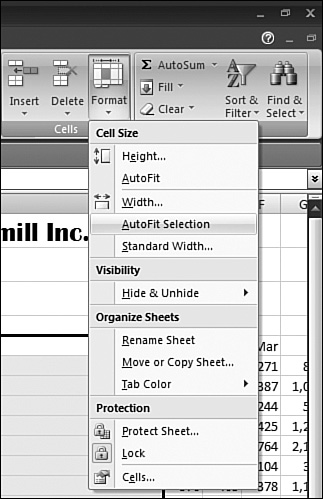
• Autofit a column to all the data below the title rows—If you have a long title in the first few rows and need to autofit the column to all the data below the title rows, you use this method. You click the first cell in the data range. Then you press the End key. Next, you hold down the Shift key while pressing the Down Arrow key. This selects a contiguous range from the starting cell downward. Now, you select the Cells section of the Home ribbon and then select Format, AutoFit Selection, as shown in Figure 32.21. If you were a power user in Excel 2003 or before, you might remember this method as Alt+O+C+A. This legacy keyboard shortcut still works.

Figure 32.21. The traditional column width command can be found in the Format drop-down in the Cells group of the Home ribbon.

Using Merge and Center

In general, merged cells are bad. If you have a merged cell in the middle of a data table, you will be unable to sort the data. You will be unable to cut and paste data unless the same cells are merged. However, it is okay to use merged cells as a title to group several columns together.

In Figure 32.22, the Consumer and Professional headings correspond to the columns B:F and G:K, respectively. It would be appropriate to center each heading above its columns.

Figure 32.22. Because the Row 2 categories are not part of the data table and would never need to be sorted, it is okay to merge and center those cells.

To merge and center cells, you follow these steps:

1. Click in the cell that contains the value to be centered and drag to select the entire range to be merged. In this example, you would click in Cell B2 and drag to Cell F2. The result is that B2 is the active cell, and B2:F2 is selected.
2. From the Home ribbon, select Alignment, Merge and Center and then select Merge and Center again, as shown in Figure 32.23.

   Figure 32.23. Select Merge and Center from the drop-down.

   

3. Repeat steps 1 and 2 for any other column headings.
4. Optionally, apply an outline border around the merged cells.

Note that after you merge the cells, the entire range becomes one cell. In Figure 32.24, the word Consumer is in an ultra-large Cell B2. In this worksheet, cells C2, D2, E2, and F2 no longer exist.

Figure 32.24. Columns are visually grouped into product lines by the merged cells.

Rotating Text

Vertical text is difficult to read. However, there are times when space considerations make it advantageous to use vertical text. In Figure 32.25, for example, the names in Row 5 are much wider than the values in the rest of the table. If you use Format, Autofit Selection, the report is too wide.

Figure 32.25. The headings are much wider than the data. Vertical text could solve the problem.

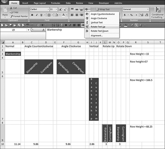
In the Alignment tab of the Home group, an Orientation drop-down offers five variations of vertical text. Figure 32.26 compares the five available options. Although the Angle options look great, they only reduce the column width by 12%. Vertical Text reduces the column width by 75% but takes far more vertical space. The option Rotate Text Up reduces the column width by 73% and takes up less than half the vertical space of the Vertical Text option.

Figure 32.26. Of the five options, the Rotate Text options take up the least space.

If you need more control over the text orientation, you can select the Alignment option in the drop-down to display the Alignment tab of the Format Cells dialog. This tab allows rotation from 90 degrees to -90 degrees, in 1 degree increments, as shown in Figure 32.27.

Figure 32.27. The Alignment option allows 182 different orientation settings.

Formatting with Styles

Instead of using the settings in the Font group of the Home ribbon, you could format a report by using the built-in cell styles. Cell styles have been popular in Word for over a decade. They have been available in Excel, but because they were not given a spot on the Formatting toolbar, few people took advantage of them.

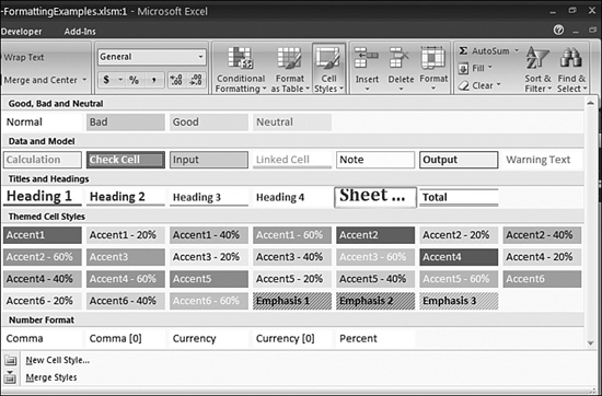
Figure 32.28 shows the styles available when you select Styles, Cell Styles in the Home ribbon.

Figure 32.28. The Cell Styles gallery offers various built-in cell styles.

An advantage to using cell styles is that you can quickly convert the look and feel of a report by choosing from the themes on the Page Layout ribbon. Figure 32.29 shows 1 of the 20 available themes applied to the report.

Figure 32.29. When you choose a new theme, a report formatted with cell styles takes on a new look.

The Cell Styles gallery offers a menu item to add additional styles to a workbook. Using cell styles provides an interesting alternative to the traditional method of formatting.

Other Formatting Techniques

You have the basics for formatting cells and worksheets. The rest of this chapter provides an overview of various formatting tips and tricks. These techniques discuss how to mix formatting within a single cell, wrap text in several cells, and use cell comments.

Formatting Individual Characters

Occasionally, you might find yourself entering a short memo on a worksheet. This might occur as an introduction or as instructions to a lengthy workbook. Although Excel is not a full-featured word processor, it can do a few word processing tricks.

One trick is to highlight individual characters in a cell in order to add emphasis or to make them stand out. You can do this to any cell that does not contain a formula. In Figure 32.30, for example, text has been typed in Column A and allowed to extend over the edge of the column into Columns A:J. One word in Row 4 is in a bold, underlined, red font.

Figure 32.30. You can change the formatting for individual characters in a cell by selecting those characters in the formula bar.

To format individual characters, you follow these steps:

1. Display the Home ribbon.
2. Select the cell that contains the characters to be formatted.
3. Press the F2 key to edit the cell
4. Using the mouse, highlight the characters in the formula bar.
5. Although most of the ribbon is grayed out, the options for font size, color, underline, bold, italics, and font name are available in the Font group of the Home ribbon. Apply any formatting, as desired, from this group.
6. If the changes are not visible in the formula bar, press Enter to accept the changes in order to preview them.

Changing the Default Font

Excel offers a default font setting to be used for all new workbooks. With the Excel 2007 paradigm of themes, the default font for new workbooks is initially the generic value of BODY FONT. This is not an actual font; it instead refers to the main font used by the current theme.

To change your default font for all new workbooks, you follow these steps:

1. The menu for changing the default font does not offer Live Preview of the fonts. Therefore, go to the Font section of the Home ribbon and select the Font drop-down to inspect the available fonts in their actual styles. Find the name of the font you want to use.
2. From the Office icon menu, choose Excel Options. The Excel Options dialog appears.
3. Click the Popular category in the left margin.
4. In the second section, When Creating New Workbooks, choose the Use This Font drop-down. Select the font name you chose in step 1.
5. Click OK to close the Excel Options dialog.
6. Close and restart Microsoft Excel for the changes to take effect.

The default font setting only has an effect in new workbooks. It does not affect workbooks previously created.

Wrapping Text in a Cell

You might have one column in a table that contains long, descriptive text. If the text contains several sentences, it would be impractical to make the column wide enough to include the longest value in the column. Excel offers the capability to wrap text on a cell-by-cell basis to solve this problem.

When you wrap text, one annoying feature of Excel becomes evident. All cells in Excel are initially set to have their cell contents aligned with the bottom of the cell. You probably don’t notice this because most cells in Excel are the same height. When you wrap text, however, the cell heights double or more, and it becomes very evident that the bottom alignment looks strange in this situation. To correct this problem, you follow these steps:

1. Decide on a reasonable column width for the column that contains the descriptive text. If you try to wrap text in a column that is only 8 points wide, you will be lucky to fit one word per line. If you have the space, a width of at least 24 will allow suitable results for the text wrapping.
2. From the Cells section of the Home ribbon, select Format, Column Width. Choose a width of 24 or higher.
3. Select the cells in the column to be wrapped.
4. From the Home ribbon, select Alignment, Wrap Text.
5. If the rows are too tall, you will have a tendency to grab the right edge of the column and drag it outward to make the description column wider. A long-standing bug causes Excel to not automatically resize the row heights after this step. You must select the Cells section of the Home ribbon and then select Format, Autofit to resize the row height after adjusting the column width.
6. Select all cells in the table.
7. From the Home ribbon, select Alignment, Top Align. The values in the other columns now align with the top of the descriptive text.

Figure 32.31 shows a table where the descriptions in Column B have had their text wrapped and all the cells are top-aligned.

Figure 32.31. After wrapping text in a column, you should top-align all columns.

Justifying Text in a Range

When using Excel as a word processor to include a paragraph of explanatory body copy in a worksheet, you usually have to decide where to manually break each line.

Excel offers a command that reflows the text in a paragraph in order to fit a certain number of columns.

You need to do some careful preselection work before invoking the command. You follow these steps:

1. Ensure that your text is composed of one column of cells that contain body copy. It is fine if the sentences extend beyond one column, but the text should be arranged so that the left column contains text and the remaining columns are blank.
2. Ensure that the upper-left cell of your selection starts with the first line of text.
3. Ensure that the selection range is as wide as you want the finished text to be.
4. If your sentences currently extend beyond the desired width, Excel requires more rows in order to wrap the text. Include several extra rows in the selection rectangle. Figure 32.32 shows a suitable-sized selection range.

   Figure 32.32. You need to select more rows than necessary. The number of columns selected determines the width of the final text.

   

5. From the Home ribbon, select Editing, Fill, Justify. Excel flows the text so that each line is shorter than the selection range. Figure 32.33 shows the result.

Figure 32.33. Excel flows the text to fit the width of the original selection.

Adding Cell Comments

Cell comments can contain a few sentences or paragraphs to explain a cell. Although the default is for all comments to use a yellow sticky-note format, you can customize comments with colors, fonts, or even pictures.

In the default case, a comment causes a red triangle to appear in a cell. If you hover over the triangle, the comment appears. Alternatively, you can request that comments be displayed all the time. This creates an easy way to add instructions to a worksheet.

You follow these steps to insert a comment, format it, and cause it to be displayed continuously:

1. Select a cell to which you would like to add a comment.
2. Select Review, Comments, New Comment or right-click the cell and choose New Comment.
3. The default comment starts with your name in bold on line 1 and the insertion point on line 2. To remove your name from the comment, backspace through your name and then press Ctrl+B to turn off the bold.
4. Type instructions to the person using the worksheet. You can make the instructions longer than the initial size of the comment. (A comment can contain more than 2,000 words of body copy.)
5. After entering the text, click the resize handle in the lower-right corner of the comment. Drag to allow the comment to fit the text.
6. The selection border around the comment can either be made of diagonal lines or dots. If your selection border is diagonal lines, click the selection border to change it to dots.
7. Right-click the selection border and choose Format Comment. The Format Comment dialog appears.
8. In the Format Comment dialog, change the font, alignment, colors, and so on as desired. The Transparency setting on the Colors and Lines tab allows the underlying spreadsheet to show through the comment. If you choose the Fill Color drop-down, you can select Fill Effects and insert a picture as the background in the comment.
9. Click OK to return to the comment.
10. Right-click in the cell and choose Show/Hide Comments. This causes the comment to be permanently displayed on the worksheet.
11. To reposition the comment, click the comment. Drag the selection border to a new location.

Figure 32.34 shows a comment that has been formatted, resized, and set to be displayed.

Figure 32.34. Cell comments can provide instructions or tips for people who use your spreadsheet.

Copying Formats

Excel worksheets tend to have many similar sections of data. After you’ve taken the time to format the first section, it would be great to be able to copy the formats from one section to another section. Excel 2007 offers two methods for doing this: pasting formats and using the Format Painter icon.

Pasting Formats

An option on the Paste Special dialog allows you to paste only the formats from the Clipboard. The rules for copying and pasting formats are as follows:

• If your original selection is one cell, you can paste the formats to as many cells as you want.
• If your original selection is one row tall and multiple cells wide, you can paste the formats to multiple rows, and the final paste area will be as wide as the original copied range.
• If your original selection is one column wide and multiple cells tall, you can paste the formats to multiple columns, and the final paste area will be as tall as the original copied range.
• If your original selection is multiple rows tall and multiple columns wide, you can only paste the formats to an identically sized range. You select the upper-left corner of the range before pasting. Excel expands the selection to match the original size.

You follow these steps to copy formats:

1. Select a formatted section of a report. This might be one cell, one row of cells, or a rectangular range of cells.
2. Press Ctrl+C to copy the selected section to the Clipboard.
3. Select an unformatted section of your worksheet. If your selection in step 1 is a rectangular range, you can select just the top-left cell of the destination range.
4. From the Home ribbon, select Clipboard, Paste, Paste Special. The Paste Special dialog appears.
5. In the Paste section of the dialog, choose Formats, as shown in Figure 32.35.

   Figure 32.35. The Formats option in the Paste Special dialog copies cell formatting without affecting values or formulas.

   

6. Click OK. The formats from the original section are pasted to the new section. None of the values or formulas in the destination range are changed.
7. If you have multiple target destinations to format, repeat steps 3 through 6 as needed.

The disadvantage of using the Paste Special Formats method is that it does not change column widths. After the formats are copied from B:F to H:L in Figure 32.36, notice that Columns I:K did not pick up the narrower column widths from the source columns. This problem can be solved by using the Format Painter tool, described in the next section.

Figure 32.36. Pasting formats copies formats but does not resize columns.

Using the Format Painter

The Format Painter icon appears in the Clipboard group of the Home ribbon. The prominent location of the icon might encourage you to attempt to use this feature. The Format Painter is still tricky to use.

To copy a format from a source range to a destination range, you follow these steps:

1. Select the source range. If you want to copy column widths, the source range must include complete columns.
2. Click the Format Painter icon once in the Clipboard group of the Home ribbon. The mouse icon changes to a plus and a paintbrush.
3. Immediately use the mouse to click and drag to select a destination range. If the source range was five columns wide, the destination range should also be five columns wide.
4. If you accidentally click somewhere else or click the wrong size range, undo and start over.

The new ToolTip for the Format Painter icon advertises a little-known feature of the Format Painter: You can copy a format to many different ranges. To do this, you follow these steps:

1. Select the source range.
2. Double-click the Format Painter icon.
3. Click a new destination range. The format is copied.
4. Repeat step 3 as many times as you want.
5. When you are done formatting ranges, press Esc or single-click the Format Painter icon to turn off the feature.

Copying Formats to a New Worksheet

There is an easy way to make a copy of a worksheet. This method is better than creating a new worksheet and copying formats from the original sheet to the new sheet. Among its advantages are the fact that column widths and row heights are copied and page setup settings are copied.

To copy a worksheet within the current workbook, you follow these steps:

1. Activate the worksheet to be copied.
2. Hold down the Ctrl key. Click the worksheet tab and drag it to a new location. A new sheet is created with a strange name, such as Sheet3 (2).
3. Right-click the sheet tab and choose Rename. The cursor moves to the tab, which is now editable.
4. Type a new name and press Enter. The tab has a new name.

To copy a worksheet to a new workbook, you follow these steps:

1. Activate the worksheet to be copied.
2. Right-click the sheet tab. Choose Move or Copy to display the Move or Copy dialog.
3. In the To Book drop-down, choose (new book).
4. Click Create a Copy.
5. Click OK. The single worksheet is copied to a new workbook.