
Chapter 20. Understanding Formulas
In this chapter
Getting the Most from This Chapter 386
Entering Your First Formula 388
Three Methods of Entering Formulas 395
Entering the Same Formula in Many Cells 398
Copying a Formula by Using the Table Tool 402
Excel’s forte is performing calculations. When you use Excel, you typically use a combination of cells with numbers and cells with formulas. After you design a spreadsheet to calculate something, you can easily change the numbers used in the assumption cells and then watch Excel instantly calculate new results.
Getting the Most from This Chapter
Don’t skip this entire chapter, because one particular trick in this chapter will save you daily frustration.
I regularly entertain accountants and auditors with my Power Excel program. While this program is a fun, laughter-filled tour through the inside tricks of Microsoft Excel, I do know that people are learning new things along the way.
I call them “gasp moments.”
Imagine this setting: I am in front of 200 managerial accountants—these are people who have Excel open 40 hours a week. You can generally figure that these folks are super-efficient with Excel. For any trick that I show, it might be already in the arsenal of half to three-quarters of the room. I will see a lot people nodding their heads and see an expression of surprise on a portion of the attendees.
Universally, though, there are a few tricks that get a universal gasp—perhaps 90% of the people never knew the trick and realize just how powerful it is. I thrive on the gasp moments.
I understand that everyone reading this book believes that they know Excel formulas. And, to a certain extent, this chapter is mostly a primer for the person who is new to Excel. However, even the most astute person using Excel should check out these sections of the chapter:
- Everyone should read “Copying a Formula by Double-Clicking the Fill Handle.” Somehow, most people have learned to drag the fill handle to copy a formula. This leads to horrible frustration on long data sets, as you go flying past the end of the data. This simple but powerful trick is the one that universally amazes attendees of my seminar.
- Honestly answer this question: Do you really understand the difference between cell H1 and cell $H$1? If you think the latter has anything to do with currency, you need to thoroughly review “Overriding Relative Behavior—Absolute Cell References.” This isn’t a trick, but one of the fundamental building blocks to building Excel worksheets. I would say that 5% of the people in a Power Excel seminar did not understand this, and perhaps 30% of the people in a community computer club presentation did not understand this. If you don’t know when and why to use the dollar signs, you are in good company with 20 million other people using Excel. It is worth your time to learn this essential technique.
- Finally, I can predict someone’s age by how they enter formulas. There are three ways, and I believe that my preferred way is the best. I probably won’t convince you to change, but if you understood my way, you would be able to enter formulas far faster than the other two ways. To get a good understanding of the alternatives, read “Three Methods of Entering Formulas.”
Introduction to Formulas
In Chapter 7, Table 7.1 shows a list of changed limits in Excel. A few of these limits relate specifically to formulas. For example, the number of characters in a formula increased from 1,024 to 8,192. The number of levels of nesting for IF functions increased from 7 to 64. Thanks to Excel 2007’s improved limits, you can calculate almost anything with a formula in Excel.
This chapter and Chapter 21, “Doing Cool Tricks with Formulas,” deal with formula basics. Chapters 22, “Understanding Functions,” through 27, “Using Math and Engineering Functions,” introduce adding functions to your formulas. Chapter 28, “Connecting Worksheets, Workbooks, and External Data,” introduces formulas that calculate data found on other worksheets or in other workbooks. Chapter 29, “Using Super Formulas in Excel,” provides interesting examples, such as 3D formulas and the all-powerful array formulas.
Note
The need to recalculate case studies at M.I.T. led Dan Bricklin to invent the first spreadsheet program, VisiCalc.
Because of the record-oriented nature of spreadsheets, you can generally build a formula once and then copy that formula to hundreds or thousands of cells without changing anything in the formula.
Tip From
![]()
Designing a formula that can be written once and then copied to a rectangular range of data is a fantastic way to make your use of Excel more efficient.
Formulas Versus Values
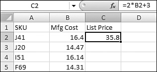
When looking at an Excel grid, you can’t tell the difference between a cell with a formula and one that contains numbers. To see if a cell contains a number or a formula, you select the cell. Look in the formula bar. If the formula bar contains a number, as shown in Figure 20.1, you know that it is a static value. As shown in Figure 20.2, if the formula bar contains a formula (most formulas start with =), you know that the number shown in the grid is the result of a formula calculation.
Figure 20.1. The formula bar reveals whether a value is a static number or a calculation. In this case, Cell B2 contains a static number.

Figure 20.2. In this case, Cell B2 contains the result of a formula calculation. A formula usually starts with an equals sign.

Entering Your First Formula
Your first formula was probably a SUM function, entered with the AutoSum button. However, for this discussion, I am talking about a pure mathematic formula that uses a value in a cell, added, subtracted, divided, or multiplied by a number or another cell.
There are billions of variations of formulas that can be used. Everyday life throws situations at you that can be solved with this type of formula. Keep these important points in mind as you start tinkering with your own formulas:
- Every formula starts with an equal sign.
- Entering formulas is then just like typing an equation in a calculator with one exception (see the next point).
- If one of the terms in your formula is already stored in a cell in Excel, you can point to that cell’s address instead of typing in the number in that cell. Using this method will allow you to change the value in one cell and then watch all of the formulas recalculate.
To illustrate these points, watch the steps to building a basic formula for a specific example.
In Figure 20.3, you want to enter a formula to calculate a target sales price. Cell B2 shows the product cost. In Column C, you want to calculate list price as two times the cost plus $3.
Figure 20.3. The formula in Cell C2 recalculates if the value in Cell B2 changes.
To enter a formula, follow these steps:
- Put the cell pointer in Cell C2.
- Type an equal sign. The equal sign tells Excel that you are starting a formula.
- Type 2*B2. This indicates that you want to multiply two times the value in cell B2.
- Type +3 to add three to the result. There should be no spaces in the formula. If your formula reads =2*B2+3, proceed to step 5. Otherwise, use the backspace key to correct the formula.
- Press Enter. Excel calculates the formula in Cell C2.
By default Excel usually moves the cell pointer down or to the right after you finish entering a formula. You should move the cell pointer back to Cell C2 to inspect the formula, as shown in Figure 20.3. Note that Excel shows a number in the grid, but the formula bar reveals the formula behind the number.
The Relative Nature of Formulas
The formula =2*B2+3 really says “multiply two by the cell immediately to the left of me and add three.” If you need to put this formula in Cells C3 to C999, you do not need to re-enter the formula 996 times. You can simply copy the formula and paste it to all the cells. As you copy, Excel copies the essence of the formula: “Multiply two by the cell to the left of me and add three.” As you copy the formula to Cell C3, the formula becomes =2*B3+3. Excel handles all this automatically.
Figure 20.4. After you paste the formula, Excel automatically updates the cell reference to point to the current row.
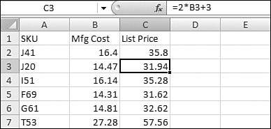
Excel’s ability to change B2 to B3 in the formula is called relative referencing. This is the default behavior of a reference. Sometimes, you do not want Excel to change a reference as the formula is copied, as explained in the next section.
Overriding Relative Behavior: Absolute Cell References
Excel’s ability to change a formula as it is copied is what makes spreadsheets so useful. However, there are times when you need part of a formula to always point at one particular cell. This happens a lot when you have a setting at the top of the worksheet, such as a growth rate or a tax rate. It would be nice to change this cell once and have all of the formulas use the new rate.
The following example sets up a sample worksheet that exhibits this problem and shows you how to use an arcane notation style to easily solve the problem. When you see a reference with two dollar signs, for example $G$1, this indicates an absolute reference to G1.
Say that you have a sales tax factor in a single cell at the top of a worksheet. After you enter the formula =C2*G1, it accurately calculates the tax in Cell D2, as shown in Figure 20.5.
Figure 20.5. This formula works fine in Row 2.
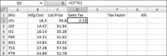
However, when you copy the same formula to Cell C3, you get a zero as the result. As you can see in Figure 20.6, Excel correctly changed Cell C2 to C3 in the copied formula. However, Excel also changed G1 to G2. Because there is nothing in G2, the calculation predicts a zero.
Figure 20.6. This formula fails in Row 3.

Because the sales tax factor is only in G1, you really want Excel to always point to G1. To make this happen, you need to build the original formula as =C2*$G$1. The two dollar signs tell Excel that you do not want to have the reference change as the formula is copied. The $ before the G freezes the reference to always point to Column G. The $ before the 1 freezes the reference to always point to Row 1. Now, when you copy this formula from Cell D2 to other cells in Column D, Excel changes the formula to =C3*$G$1.
Figure 20.7. The dollar signs in the formula make sure that the copied formula always points to Cell G1.

To recap, a reference with two dollars signs is called an absolute reference.
Using Mixed References to Combine the Features of Relative and Absolute References
In a number of situations, you might want to build a reference that has only one dollar sign. For example, in Figure 20.8, you want to use the monthly bonus rate in Row 3, but you want to allow the column to change. The formula for Cell C19 would be =C6*C$3.
Figure 20.8. By having the dollar sign before the 3 in C$3, you lock the reference to Row 3 but allow the formula to point to Columns D, E, and so on as you copy the formula.
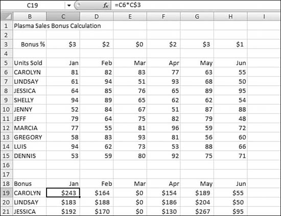
When you copy this formula, it always points to the bonus amount in Row 3, but the remaining elements of the formula are relative. For example, the formula in D21 is =D8*D$3, which multiplies Jessica’s February sales by the February bonus rate.
There are two kinds of mixed references. One mixed reference freezes the row number and allows the column letter to change. The other mixed reference freezes the column letter, but allows the row number to change. No one has thought up clever names to distinguish between these references—they are both simply called mixed references.
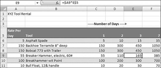
As another example of the other kind of mixed reference, in Figure 20.9, you want a single formula to multiply the daily rate from Column A by the number of days in Row 4. This formula requires both kinds of mixed references.
Figure 20.9. You can create a formula by using a combination of dollar signs to allow Cell C6 to be copied to all cells in the table.

In this case, you want the Cell A6 reference to always point to Column A, even as the formula is copied to the right. The A6 portion of the formula should therefore be entered as $A6. You also want the C5 portion of the formula to always point to Row 5, even as the formula is copied down the rows. The C5 portion of the formula should therefore be entered as C$5.
Using the F4 Key to Simplify Dollar Sign Entry
In the preceding section, you had to enter quite a few dollar signs in formulas. But you do not have to type the dollar signs! Immediately after entering a reference, you can press the F4 key to toggle the reference from a relative reference to an absolute reference that automatically has the dollar signs before the row and column. If you continue pressing F4, the reference toggles to a mixed reference with a dollar sign before the row number and then to a mixed reference with a dollar sign before the column letter. Pressing F4 again returns the reference to a relative reference. I find that it is easier to choose the right reference by looking at the various reference options offered by the F4 key.
The following sequence walks through how the F4 key works while you are entering a formula. This particular example was chosen because it requires two different types of mixed references.
The important concept is that you start pressing F4 after typing a cell reference but before you type a mathematical operator.
- Type =A6 (see Figure 20.10).
Figure 20.10. This is a relative reference: A6 without any dollar signs.

- Before typing the asterisk to indicate multiplication, press the F4 key. On the first press of F4, the reference changes to =$A$6, as shown in Figure 20.11.
Figure 20.11. After you press F4 once, the reference changes to an absolute reference, with two dollar signs.

- Press the F4 key again. The reference changes to A$6 to freeze the reference to Row 6, as shown in Figure 20.12.
Figure 20.12. You press F4 again to switch to a mixed reference with the row number locked.

- Press F4 one more time. Excel locks just the column, changing the reference to =$A6, as shown in Figure 20.13. This is the version of the reference that you want.
Figure 20.13. You can press F4 again to switch to a mixed reference with the column letter locked.

Note
After you press F4 again, Excel returns the reference to the relative state A6. As you continue to press F4, Excel toggles between the four modes. It is fine to toggle between them all and then choose the correct one. If you accidentally toggle past the $A6 version, you can just keep pressing F4 until the correct mode comes up again.
- To continue the formula, type an asterisk to indicate multiplication and then click Cell C5 with the mouse. At the point shown in Figure 20.14, you would have to press F4 twice to change C5 to a reference that locks only the row (that is, C$5).
Figure 20.14. After clicking C5 with the mouse, you need to press F4 twice to change this reference.

- Press Enter to accept the formula.
- When you copy the formula from Cell C6 to the range C6:H36, the formula automatically multiplies the rate in Column A by the number of days in Row 5. Figure 20.15 shows the copied formula in Cell E9. The formula correctly multiplies the 55-dollar rate in Cell A9 by the three days figure in Cell E5.
Figure 20.15. By using the correct combination of row and column mixed references, you can enter this formula once and successfully copy it to the entire rectangular range.
Using F4 After a Formula Is Entered
The F4 trick described in the preceding section works immediately after you enter a reference. If you try to change Cell A6 after you type the asterisk, pressing the F4 key has no effect.
You can still use F4 in this case, however. You simply click somewhere in the formula bar adjacent to the characters A6. Pressing F4 now adds dollar signs to that reference.
Using F4 on a Rectangular Range
Some functions allow you to specify a rectangular range. For example, in Figure 20.16, you would like to enter a formula to calculate month-to-date sales. One formula in Cell C29 is =SUM(B2:B29). To be able to copy this formula, you need to change the formula to be =SUM(B$2:B29).
Figure 20.16. Using F4 at this point will never produce the desired result.
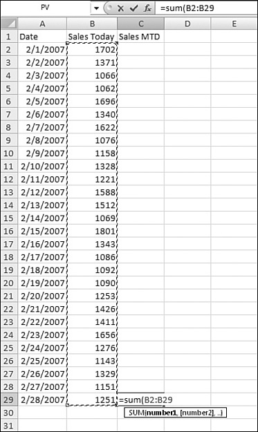
At the point in the figure, you might be tempted to press the F4 key. However, pressing F4 at this point would convert the reference to the fully absolute range $B$2:$B$29. Continuing to press F4 would toggle to B$2:B$29, then $B2:$B29, then B2:B29. Excel does not even attempt to go through the other 12 possible combinations of dollar signs in order to eventually offer B$2:B29.
In this case, you need to click the insertion point just before, just after, or in the middle of the characters B2 in the formula bar. If you then press F4, you toggle through the various dollar sign combinations, just on the B2 reference. Pressing F4 twice results in the proper combination, as shown in Figure 20.17.
Figure 20.17. Using F4 is tricky when your reference is a rectangular range—you must click in to the formula.

Three Methods of Entering Formulas
In the examples in the previous sections, you entered a formula by typing it. Although you generally need to start a formula by typing the equals sign (or the plus sign), after that point, you have three options:
- Type the complete formula as described above.
- Type operator keys, but use the mouse to touch cell references. I will call this the mouse method.
- Type the operator keys, and use the arrow keys to specify the cell references by navigating to the cells. I will call this the arrow key method.
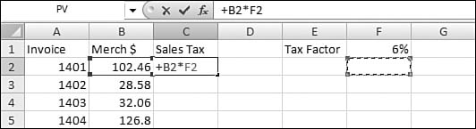
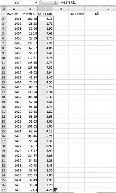
Assume that in Figure 20.18, you would like to multiply the merchandise total in Cell B2 by the sales tax rate in Cell F1.
Figure 20.18. There are three methods for entering the formula =B2*$F$1.

Mouse Method for Entering Formulas
If you started using computers after the advent of Microsoft Windows 3.1, it is likely that you use the mouse method for entering formulas. This method is intuitive, but it requires you to move your hand between the keyboard to the mouse several times, as in this example:
- Type =.
- Click in Cell B2.
- Type *. (If you have a desktop keyboard, you can use the asterisk key on the numeric keypad to avoid pressing the Shift key.)
- Click in Cell C1.
- Press F4 to add the dollar signs.
- Press Enter. This usually moves the cell pointer to Cell C3.
This method requires only four keystrokes, but it requires you to move to the mouse twice. Moving to the mouse is the slowest part of entering formulas, but this method is easier than typing the entire formula if you are not a touch typist.
Entering Formulas Using the Arrow Key Method
The arrow key method is popular with people who started using spreadsheets in the days of Lotus 1-2-3 release 2.2. It is worthwhile to learn this method because it is incredibly fast. Almost all the formula entry can be accomplishing using keys on the right side of the keyboard. Here’s how it works:
- In Cell C2 type +. (If you have a desktop keyboard, you can use the plus key on the numeric keypad to avoid pressing the Shift key.)
- Press the left-arrow key to move the flashing cell border to Cell B2. Note that the active cell (that is, with a solid border) is still Cell C2. The flashing border is like a second cell pointer that you can use to point to the correct cell for the formula. As shown in Figure 20.19, the temporary formula in the formula bar reads +B2.
Figure 20.19. By using the arrow keys during formula entry, you create a flashing border that you can use to navigate to a cell reference.

- To add Cell B2 as the correct reference in the formula, press either an operator key (for example, *, +), a parenthesis, or the Enter key. In this case, type *.
- Note that the dashed cell pointer disappears, and the focus is now back to the original cell, C2.
- Press the right-arrow key three times. The flashing cell border moves to D2, E2, and then F2. With each keypress, the temporary formula in the formula bar shows an incorrect formula (+B2*D2, +B2*E2, and +B2*F2). Figure 20.20 shows what the screen looks like after you press the right-arrow key three times.
Figure 20.20. After step 4, the focus moves to the original cell. Thus, you only have to press the right-arrow key three times instead of four times to arrive at Cell F2.
- Type the up-arrow key to move the flashing cell border to the correct location, Cell F1.
The temporary formula in the formula bar now shows +B2*F1. - Press the F4 key to add dollar signs to the F1 reference.
- Press Ctrl+Enter to accept the formula and keep the cell pointer in Cell C2.
Using this method requires 10 keystrokes, with no trips to the mouse. You can enter formulas that have no absolute references, mixed references, parentheses, or exponents by using just the arrow keys and the keys on the numeric keypad.
Tip From
![]()
Even if you are mouse-centric, you should try this method for half a day. When you get the feel for navigating by using the arrow keys, you can enter formulas much faster by using this method.
Note
Officially, every formula must start with an equals sign. However, to make former Lotus 1-2-3 users comfortable, Excel allows you to start a formula with a plus sign. Power Excel users have discovered that using a plus sign allows you to start a formula by typing on the numeric keypad. Because I routinely start formulas with the plus sign, I am often asked why I start with =+ instead of just =. Even though the formulas appear that way onscreen, I don’t actually enter the =. When a formula starts with a plus sign, Excel adds an equals sign and does not remove the plus sign, so you end up with a formula that looks like =+B2*$F$1.
Entering the Same Formula in Many Cells
So far in this chapter, you’ve entered a formula in one cell and then copied and pasted to get the formula in many cells. There are three alternate strategies:
- Preselect the entire range where the formulas need to go. Enter the formula for the first cell and press Ctrl+Enter to simultaneously enter the formula in the entire selection.
- Enter the formula in the first cell and then use the fill handle to copy the formula.
- The new method in Excel 2007 is to define the range as a table. New formulas will be copied automatically.
Copying a Formula by Using Ctrl+Enter
This strategy works when you are entering formulas for a screen full or two of data:
- If you have just a few cells, select them before entering the formula.
- Click in the first cell and drag down to the last cell, as shown in Figure 20.21. Notice from the name box that the active cell is the first cell.
Figure 20.21. You click in the first cell and drag down to the last cell to select a range with the first cell as the active cell.

- Enter the formula by using any of the three methods described earlier in this chapter. Even if you use the arrow key method, Excel keeps the entire range selected. Figure 20.22 shows the formula after you press F4 to convert the F1 reference to $F$1.
Figure 20.22. Even with a large range selected, the formula is built only in the active cell.

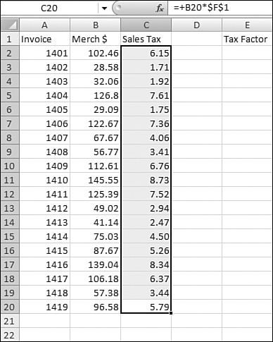
- At this point, you would normally press Enter to complete the formula. Instead, press Ctrl+Enter to enter this formula in the entire selected range. Note that Excel does not enter =B2*$F$20 in each cell. Instead, it converts the formula as if it were copied to each cell. Figure 20.23 shows the formula in Cell C20.
Figure 20.23. Pressing Ctrl+Enter tells Excel to enter the formula in the active cell and to also copy it to the rest of the selection.
Copying a Formula by Dragging the Fill Handle
If you want to enter a formula in one cell and then copy it to the other cells in a range, you can use the fill handle (that is, the square dot in the lower-right corner of the cell pointer). There are two ways to use the fill handle:
- Drag the fill handle.
- Double-click the fill handle.
The dragging method works fine when you have less than one screen full of data:
- Enter the formula in Cell B2.
- Press Ctrl+Enter to accept the formula and keep the cell pointer in Cell B2.
- Click the fill handle. You know that you are above the fill handle when the mouse pointer changes to a thick plus sign, as shown in Figure 20.24. Drag the mouse down to the last row of data (in this case, Cell C20).
Figure 20.24. You can copy a formula by clicking and dragging the fill handle.

- When you release the mouse button, the original cell is copied to all the cells in the selected range.
This method is fine for copying a formula to a few cells. However, if you have thousands or hundreds of thousands of cells, it is annoying to drag to the last row. Invariably, as the scroll effect speeds up, you end up flying past the last row. In such a case, it is easier to copy a formula by double-clicking the fill handle.
Copying a Formula by Double-Clicking the Fill Handle
In most datasets, double-clicking the fill handle is the fastest way to copy the formula. While you will love this method, you need to understand a few shortcomings that can hamper the method when an adjacent column has blank cells amongst the data.
Figure 20.25 shows a table that has hundreds of rows of data. You want to copy the formula from Cell C2 down to all the rows of data in Column B.
Figure 20.25. Dragging the fill handle is frustrating in a table that has hundreds of rows. The double-click method will end that frustration.

In this particular case, Cell B2 is nonblank, and Column B contains a value in every row down to the end of the data. This is the perfect condition for using the technique of double-clicking the fill handle. Follow these steps:
- Enter the formula in Cell B2.
- Press Ctrl+Enter to accept the formula and keep the cell pointer in Cell B2.
- Double-click the fill handle.
The active cell is copied down to the last row of your data, as shown in Figure 20.26.
Figure 20.26. You can double-click the fill handle to copy to the last row of your data.
The fill handle double-click method is fast. There are several arcane rules that can trip up the data, particularly if the column to the left contains a blank cell before the end of the data. Excel will be tricked into stopping the copy early because of this blank cell.
There are other rules. The fill handle can copy based on data in the adjacent column to the right or even data in the current column.
You should always type End and then the down arrow to make sure that the formula was copied far enough.
For a complete discussion of the arcane rules, see the Excel Troubleshooting section at the end of this chapter.
Copying a Formula by Using the Table Tool
The table tool is a new feature in Excel 2007. When you use this tool, if you tell Excel that your current dataset is a table, Excel automatically copies new formulas down to the rest of the cells in the table.
Figure 20.27 shows an Excel worksheet that has headings at the top and many rows of data below the headings. Notice the blank Cell C15, which would normally trip up the fill handle double-click method.
Figure 20.27. This is a typical worksheet in Excel.

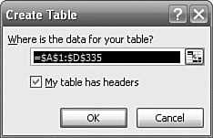
To define a range as a table, select a cell within the dataset and type Ctrl+T or Ctrl+L. Excel uses its IntelliSense to guess the edges of the table. If its guess is correct, click OK in the Create Table dialog, as shown in Figure 20.28.
Figure 20.28. The Create Table dialog.
As shown in Figure 20.29, after Excel recognizes the range as a table, several changes occur:
Figure 20.29. Defining a range as a table provides formatting and powerful features such as autofilters and natural language formulas.

- The table is formatted with the default formatting. Depending on your preferences, this might include banded rows or columns.
- AutoFilter drop-downs are added to the headings.
- Any formulas that you enter use the headings to refer to cells within the table.
If you now enter a formula in the table, Excel automatically copies that formula down to all rows of the table. The entire range, starting at D3 and extending downward, flashes black momentarily. This copy works even better than the fill handle double-click method because the copy is able to go past the blank cell in Row 15.
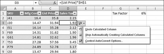
Note
As shown in Figure 20.30, there is a lightning bolt drop-down to the right of Cell D3. This drop-down offers you the opportunity to stop Excel from automatically copying the formula down.
Figure 20.30. Thanks to the new table tool in Excel 2007, a new formula entered anywhere in Column D is automatically copied to all the cells in Column D.
Troubleshooting Tip: Overcoming the Arcane Rules for Fill Handle Double-Clicking
The fill handle double-click trick is one of the best and least-known tricks. (I get a bunch of gasps whenever I show this trick in an Excel seminar.)
The problem with this method is that there are some fairly arcane rules that govern how this works. Three cells govern whether or how the double-click trick will work: the cell immediately to the left of the active cell, the cell immediately below the active cell, and the cell immediately to the right of the active cell.
In Figure 20.31, the active cell is B4. When you double-click the fill handle, Excel first looks at the three cells highlighted in blue. If all three of them are blank, Excel ignores the double-click.
Figure 20.31. Excel looks at the three cells immediately to the bottom, left, and right of the active cell.

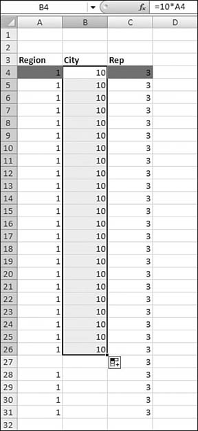
If the cell immediately below the active cell is nonblank, Excel copies the active cell down until it discovers a blank cell in the current column. In the example in the figure, this causes the formula to be copied down and overwrite the existing cell values in B4:B19, as shown in Figure 20.32.
Figure 20.32. If the cell below the active cell is nonblank, Excel copies the cell until it encounters a blank cell in the current column.

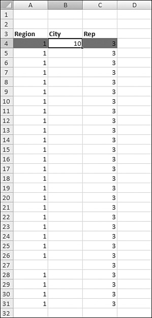
If the cell below the active cell is blank, Excel next looks to see whether the cell to the left of the cell is nonblank. In Figure 20.33, there are cells to the left and right of the active cell. Although the data in Column C is filled in to the end, there is a blank cell in the middle of the Column A data. However, because cell A5 is nonblank, Column A becomes the column that governs the action of the fill handle double-click. Excel copies the formula only until it encounters a blank cell in Column A.
Figure 20.33. Even though the data is “better” in Column C, the fact that Cell A5 is nonblank causes Excel to copy only until it encounters a blank cell in Column A.
This situation happens quite frequently: You want to copy a formula based on the adjacent column, but the column to the left has one blank cell in the midst of the data. This blank cells fools Excel, causing the copy to stop prematurely. In this situation, you can double-click the fill handle in Cell B4, and the formula in that cell is copied to B5:B26, as shown in Figure 20.34.
Figure 20.34. The fill handle double-click stops prematurely because of the blank Cell A27.
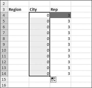
The final situation happens when only the cell to the right of the active cell is nonblank, as shown in Figure 20.35. In this case, Excel copies the cell until it encounters a blank cell in Column C.
Figure 20.35. When only the cell to the right of the active cell is nonblank, Excel copies data down until it encounters a blank cell in the column to the right of the active cell.

The ability to have the fill handle double-click trick work based on a column to the right of the active cell is useful. In this case, the cell is copied correctly to B5:B14, as shown in Figure 20.36.
Figure 20.36. The fill handle double-click method works for adjacent data—even data to the right of the active cell.
It is good to understand the arcane rules involved in the fill handle double-click trick. After you use this method, you can press the End key and then the down-arrow key to make sure Excel copied the cell to the real end of your data set.
Excel in Practice: Using the Fill Handle Double-Click Method
Blank cells in adjacent cells cause problems for the fill handle double-click method. There are situations where you need to copy a formula down a column. The column to the right is perfectly filled in without any blanks and the column to the left has many blanks.
In this case, you would prefer that Excel looks to the adjacent column on the right. However, if the first few cells to the left of the formula are nonblank, Excel will always base the copy on the column to the left.
In this case, you can solve the problem by temporarily inserting a blank column to the left of your formula. This will prevent Excel from basing the copy on the blank-ridden left column.
Here is a specific example.
Say you have a file that contains name and address information, as shown in Figure 20.37. Before you import this information to your label printing program, you need to combine the city, state, and zip code columns into a single column.
Figure 20.37. You need to convert this data to only four columns before importing to your label printing program.

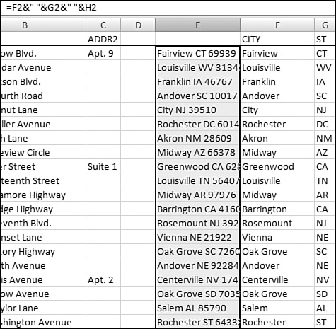
To combine City, State, and Zip into a single field, insert a blank Column D and enter the formula =E2&” “&F2&”, “&G2 in cell D2, as shown in Figure 20.38.
Figure 20.38. You would like to copy this formula by double-clicking the fill handle.

Remember the rules for the fill handle double-click method: Excel first looks in Cell D3. Because that cell is blank, Excel then looks at Cell C2.
It happens that Column C is very sparse. It is nonblank only when the person lives in an apartment. However, because Cell C2 is non-blank, Excel allows Column C to govern how far the fill handle double-click method works. Because the first blank cell in Column C is C3, Excel actually does not copy D2 at all when you double-click. However, if you remember the action shown in Figure 20.32, you realize that you could use the fill handle double-click trick if Cell C2 were blank.
To force Excel to base the copy on the data to the right, insert another temporary blank Column D. Now when you double-click the formula in Cell E2, it uses the city in Column F as the guide and successfully copies the formula to the end of the database, as shown in Figure 20.39.
Figure 20.39. Because the cell to the left of Cell E2 is blank, the double-click trick works successfully.
You can now delete the temporary Column D.