Chapter 27. Using Trig, Matrix, and Engineering Functions

In this chapter

A Brief Review of Trigonometry Basics 740

Examples of Trig Functions 750

Working with Imaginary Numbers 756

Solving Simultaneous Linear Equations with Matrix Functions 763

Examples of Engineering Functions 770

Using the Analysis Toolpack to Perform Fast Fourier Transforms (FFTs) 794

Scientists, mathematicians, and engineers, as well as high school mathematics students, will get the broadest use out of the functions in this chapter.

Even though many of the trigonometry functions might seem intimidating, I have tried to provide practical household examples for many of the functions. Anyone who has to lean a ladder up against a house can find a use for the trig functions.

The imaginary number functions might only be useful to electrical engineers, but any business analyst could make use of the techniques for solving linear equations.

Table 27.1 provides an alphabetical list of all of Excel 2007’s trig functions. Detailed examples of the functions are provided later in the chapter.

Table 27.1. Alphabetical List of Trig Functions

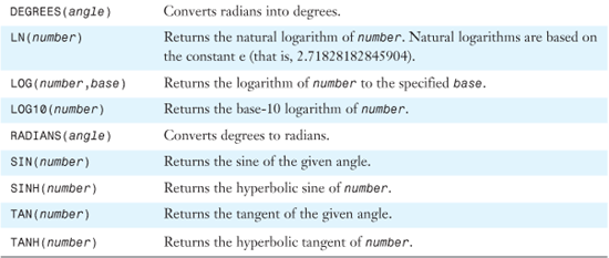
Table 27.2 provides an alphabetical list of all of Excel 2007’s matrix functions. Detailed examples of the functions are provided later in the chapter.

Table 27.2. Alphabetical List of Matrix Functions

Table 27.3 provides an alphabetical list of all of Excel 2007’s engineering functions. Detailed examples of the functions are provided later in the chapter.

Table 27.3. Alphabetical List of Engineering Functions

A Brief Review of Trigonometry Basics

There are numerous real-life examples of situations in which trigonometry can be used. In case trigonometry is just a distant nightmare for you, the following sections review some of the basics.

Radians Versus Degrees

Nonmathemeticians discuss angles in terms of degrees. Most corners of a room are at a 90-degree angle. Mathematicians discuss angles in a different measurement, called radians.

While a circle is composed of 360 degrees, it is also composed of about 6.28 radians. Each radian is equal to about 57.3 degrees. The exact relationship of degrees to radians requires you to use the mathematical constant pi (Π), which is about 3.14159. There are 2 × Π radians in a circle.

Because the trig functions were written with mathematicians in mind, they always expect the arguments to be expressed in radians.

The formula to convert degrees to radians is to multiply the degrees by PI() and divide by 180. To use this method, you would have to write formulas as shown in Cell C16 of Figure 27.1. Luckily, Excel provides the functions RADIANS and DEGREES to easily convert from one measurement to another.

Figure 27.1. The trig functions in Excel expect degrees to be in radians. These two functions convert back and forth from radians to degrees.

Syntax: DEGREES(angle)

The DEGREES function converts radians into degrees. The argument angle is the angle, in radians, that you want to convert.

Syntax: RADIANS(angle)

The RADIANS function converts degrees to radians. The argument angle is an angle, in degrees, that you want to convert.

In Figure 27.1, B2:B9 converts degrees to radians. The range B12:B14 converts radians back to degrees. The formulas in Rows 16 and 17 contrast using PI() / 180 with the RADIANS function.

Pythagoras and Right Triangles

Trigonometry relies on triangles. Figure 27.2 shows a right triangle, which is a triangle that has one 90-degree angle. In a right triangle, the side opposite the right angle is known as the hypotenuse. In a right triangle, the square of the hypotenuse is equal to the sum of the squares of the two other sides. This is frequently expressed as c^2 = a^2 + b^2.

Figure 27.2. The Pythagorean theorem allows you to figure out the length of one leg of a right triangle if you know the length of the other two legs.

If you know that the two shorter legs of a right triangle measure 3 feet and 4 feet, then you know the following:

c^2 = 3^2 + 4^2

c^2 = 9 + 16

c^2 = 25

c = SQRT(25)

c = 5

Although this formula was discovered a thousand years before Pythagoras was alive, he certainly popularized it, and it is known as the Pythagorean theorem.

One Side Plus One Angle = Trigonometry

There are three classic functions in trigonometry: sine, cosine, and tangent. These functions describe the ratio of two sides of a triangle when you know the angles of the triangle.

Consider Figure 27.3. One angle is a right angle, which is 90 degrees. If you can figure out one of the other angles and the length of one leg of the triangle, you can figure out the length of all three sides of the triangle by using Excel.

Figure 27.3. If you know one angle and the length of one side of a right triangle, you can calculate all the sides of the triangle by using trigonometry.

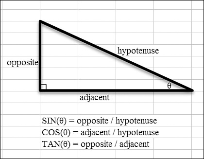
In Figure 27.3, one angle is marked θ (theta). The side across from θ is known as the opposite side. The side that is not the hypotenuse and is part of the angle θ is the adjacent side. Three classic functions describe the ratio of any two sides:

Excel offers three trig functions that allow you to find various angles or lengths of a right triangle when you know various combinations of the other angles and/or sides. The examples in this section provide some real-world examples of using trigonometry.

Using TAN to Find the Height of a Tall Building from the Ground

Suppose you would like to measure the height of a tall building from the ground. The tangent function can find the height of a right triangle if you know the length of the base and the angle to the top of the triangle. To calculate the height of a building, you could follow these steps:

1. Starting from the building, measure out 35 feet along level ground. Sight to the top of the building and determine the angle from that point on the ground to the top of the building (for example, 69 degrees). The 35-feet figure is the length of the adjacent side of the triangle. You would like to solve for the opposite side of the triangle. The TAN function describes the ratio of the opposite side to the adjacent side.
2. In a cell in Excel, enter =TAN(RADIANS(69)). This tells you that the ratio of the height of the building to the 35 feet is 2.605.
3. Because 2.605 = Opposite / Adjacent, plug in 35 for the adjacent side, to get 2.605 = Opposite / 35.
4. To solve this equation, multiply both sides by 35. The answer, as shown in Cell E8 in Figure 27.4, is that the building is more than 91 feet tall.

Figure 27.4. You can use the TAN function to find the height of this building.

Syntax: TAN(number)

The TAN function returns the tangent of the given angle. The argument number is the angle, in radians, for which you want the tangent. If your argument is in degrees, you convert it to radians by using RADIANS(degrees) or multiply it by PI() / 180.

Using SIN to Find the Height of a Kite in a Tree

Suppose your children are flying a kite. They have let out all 150 feet of string. The kite gets caught at the top of a faraway tree, as shown in Figure 27.5.

Figure 27.5. The SIN function can find the height of this tree when you know the length of the string.

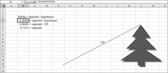
To find the height of this tree, you follow these steps:

1. Sight the angle from the end of the string to the top of the tree. It measures 29 degrees.
2. Refer to Table 27.4 earlier in this chapter. Because you know the hypotenuse and want to find the opposite side, use the SIN function.

   Table 27.4. Guide to Trig Functions

   

3. In a cell in Excel, enter =SIN(RADIANS(29)). The result is 0.484.
4. Because the sine is the ratio of the opposite side to the hypotenuse, create the formula 0.484 = Opposite / 150.
5. To solve for the opposite side, multiply both sides of the equation by 150. You find that the tree is over 72 feet tall.
6. Assess your tree-climbing skills. If you don’t currently work for Davey Tree Experts, perhaps you should decide to buy the kids a new kite.

Syntax: SIN(number)

The SIN function returns the sine of the given angle. The argument number is the angle, in radians, for which you want the sine. If your argument is in degrees, you multiply it by PI() / 180 to convert it to radians.

Using COS to Figure Out a Ladder’s Length

Every year, my wife, Mary Ellen, hires Kevin the landscaper to hang a huge holiday wreath on the second story of our house. The holidays come and go, and I find that Kevin is wintering in Florida. The ladder that I own is not long enough to reach the wreath. Much to the humor of my neighbors, I stand next to the house, with my too-short ladder, and asses the situation. Figure 27.6 shows that I am 10 feet from the house, and the angle to the wreath hanger is 55 degrees. How long of a ladder do I need to borrow from the neighbors?

Figure 27.6. The COS function can find the length of the ladder needed to reach the objective.

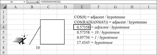
Table 27.4 (earlier in this chapter) shows that the COS function determines the relationship between the adjacent side and the hypotenuse. To find the length of the ladder, you follow these steps:

1. In Excel, enter =COS(RADIANS(55)). The result is 0.574.
2. Create the equation Adjacent / Hypotenuse = 0.574.
3. Divide both sides of the equation by 10. This tells you that the 1 / Hypotenuse is 17.43.
4. Divide both sides of the equation into 1. The result tells you that the hypotenuse is almost 17.5 feet.

I better visit Dick, the neighbor with the 18-foot ladder.

Syntax: COS(number)

The COS function returns the cosine of the given angle. The argument number is the angle, in radians, for which you want the cosine. If the angle is in degrees, you multiply it by PI() / 180 to convert it to radians.

Using the ARC Functions to Find the Measure of an Angle

If you know the lengths of two sides of a right triangle, you can determine the angles of the triangle by using trigonometry.

The ARC function converts a sine value to an angle, in radians. Say that you know the opposite side of a triangle has a length of 3 and the hypotenuse has a length of 5. The sine value is Opposite / Hypotenuse, or 0.6. You use =ASIN(0.6) to convert the sine back to the measure of the angle.

Excel provides functions to reverse all three of the basic trig functions. You use ACOS to reverse COS, ASIN to reverse SIN, and ATAN to reverse TAN.

Figure 27.8 demonstrates how to use ACOS, ASIN, and ATAN to find the angle size of a right triangle. Keep in mind that the three angles in a triangle always add up to 180. Because you know that the right angle is 90 degrees, and Figure 27.8 calculates the second angle as 37 degrees, the third angle must be 53 degrees.

Figure 27.8. The ARC functions will find an angle from the ratio of two sides of the triangle.

Syntax: ACOS(number)

The ACOS function returns the arccosine of a number. The arccosine is the angle whose cosine is number. The returned angle is given in radians, in the range 0 to Π. The argument number is the cosine of the angle you want and must be from –1 to 1. If you want to convert the result from radians to degrees, you multiply it by 180 / PI() or use the DEGREES function.

Syntax: ASIN(number)

The ASIN function returns the arcsine of a number. The arcsine is the angle whose sine is number. The returned angle is given in radians, in the range –Π / 2 to Π /2. The argument number is the sine of the angle you want and must be from –1 to 1. To express the arcsine in degrees, you multiply the result by 180 / PI().

Syntax: ATAN(number)

The ATAN function returns the arctangent of a number. The arctangent is the angle whose tangent is number. The returned angle is given in radians, in the range –Π / 2 to Π / 2. The argument number is the tangent of the angle you want. To express the arctangent in degrees, you multiply the result by 180 / PI().

Using ATAN2 to Calculate Angles in a Circle

Figure 27.9 shows a unit circle. This is a circle with a radius of 1, plotted on a Cartesian grid. The point on the right side of the circle has a value of x = 1 and y = 0. This is defined as the angle at zero degrees.

Figure 27.9. You use ATAN2 to find the angle from the x-axis to any point in Cartesian coordinates.

The point at the top of the circle has a value of y = 1 and x = 0. This is defined as the angle at 90 degrees.

Given the coordinates of any two points on the circle (actually, of any two points anywhere), you can calculate the angle by using the ATAN2 function.

Syntax: ATAN2(x_num,y_num)

The ATAN2 function returns the arctangent of the specified x- and y-coordinates. The arctangent is the angle from the x-axis to a line containing the origin (0, 0) and a point with coordinates (x_num, y_num). The angle is given in radians, between –Π and Π, excluding –Π. A positive result represents a counterclockwise angle from the x-axis; a negative result represents a clockwise angle.

This function takes the following arguments:

• x_num—This is the x-coordinate of the point.
• y_num—This is the y-coordinate of the point.

ATAN2(a,b) equals ATAN(b/a), except that a can equal 0 in ATAN2.

If both x_num and y_num are 0, ATAN2 returns a #DIV/0! error. To express the arctangent in degrees, you multiply the result by 180 / PI() or use the DEGREES function.

The formulas in Column C of Figure 27.9 find the ATAN2 of the points in Columns A and B. The result must be converted to degrees by using =DEGREES(ATAN2(A2,B2)).

Emulating Gravity Using Hyperbolic Trigonometry Functions

You could apply the trigonometry functions shown so far in this chapter to solve problems in your environment. The hyperbolic trigonometry functions, which we examine next, are far more complex. As shown in Figure 27.10, the hyperbolic cosine function, COSH, is effective at graphing the arc of a rope hung between two points.

Figure 27.10. This shape defined by COSH is also known as a catenary.

According to MathWorld.com, other uses for hyperbolic trigonometry include the following:

• Calculating the gravitational potential of a cylinder
• Calculating the rapidity of special relativity
• Calculating the profile of a laminar jet
• Calculating the Schwarzschild metric, using external isotropic Kruskal coordinates
• Emulating a uniform gravity field by a uniform acceleration, in general relativity

These are complex tasks and I won’t fill you in on the details here. If you actually need to calculate the profile of a laminar jet, head to MathWorld.com for details.

Excel offers the hyperbolic functions SINH, COSH, and TANH, as well as the reverse functions ASINH, ACOSH, and ATANH.

Syntax: SINH(number)

The SINH function returns the hyperbolic sine of a number. The argument number is any real number.

Syntax: COSH(number)

The COSH function returns the hyperbolic cosine of a number. The argument number is any real number for which you want to find the hyperbolic cosine.

In Figure 27.10, the COSH function is used in Column B to calculate the path of a rope hanging between two points.

Syntax: TANH(number)

The TANH function returns the hyperbolic tangent of a number. The argument number is any real number.

Syntax: ASINH(number)

The ASINH function returns the inverse hyperbolic sine of a number. The inverse hyperbolic sine is the value whose hyperbolic sine is number, so ASINH(SINH(number)) equals number. The argument number is any real number.

Syntax: ACOSH(number)

The ACOSH function returns the inverse hyperbolic cosine of a number. number must be greater than or equal to 1. The inverse hyperbolic cosine is the value whose hyperbolic cosine is number, so ACOSH(COSH(number)) equals number. The argument number is any real number equal to or greater than 1.

Syntax: ATANH(number)

The ATANH function returns the inverse hyperbolic tangent of a number. number must be between –1 and 1 (excluding –1 and 1). The inverse hyperbolic tangent is the value whose hyperbolic tangent is number, so ATANH(TANH(number)) equals number. The argument number is any real number between 1 and –1.

Examples of Logarithm Functions

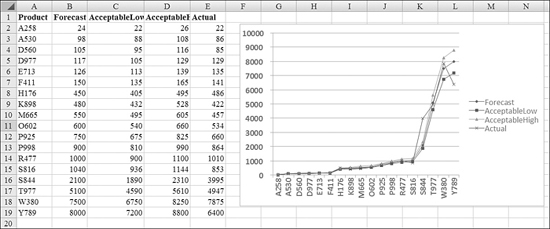
If you’ve read many of my books, you know that I used to have a day job involving forecasting and operations planning. I was constantly battling with the sales force to provide accurate sales forecasts. At the end of each month, we produced a chart to show the forecasted demand and the actual demand. If the forecast and actual were within 15% of each other, this was considered a tolerable error, and no discussion was necessary. However, for any points outside the 15% tolerance, a team would figure out why we missed the forecast and how to prevent a similar miss in future months.

The initial charts looked horrible. There were 20 products being forecasted, and the monthly demand fell by anywhere from 50 units a month to 10,000 units a month. There were only a few products above the 5,000-unit level, but those few products made it impossible to see any detail for the 17 smaller products, as shown in Figure 27.11.

Figure 27.11. No one can make out any detail for the smaller values on this chart. The scale of the two or three large products ruins the view of the smaller products.

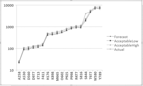
Rather than produce several different charts, our solution involved giving the y-axis of the chart a logarithmic scale.

Common Logarithms on a Base-10 Scale

In a logarithmic scale, the distance from 1 to 10 on the scale is the same as the distance from 10 to 100 and the same as the distance from 100 to 1,000 and the same as the distance from 1,000 to 10,000. Each gridline basically appears at 10^1, 10^2, 10^3, 10^4, and so on.

The resulting chart allows you to see detail for the items selling 100 units as well as the items selling 8,000 units. Figure 27.12 shows the result of converting the chart in Figure 27.11 to a chart with a logarithmic y-axis.

Figure 27.12. You can change the y-axis to show a logarithmic scale, and the detail of the smaller quantities becomes clear.

Basically, a logarithm raises a number—the base—to a certain power. In the case of the chart in Figure 27.12, each plot on the chart is located at a certain power of 10. In Figure 27.13, Columns B:E show the original numbers for the table. Columns G:J show the base-10 logarithm for the number.

Figure 27.13. The table in G:J is the base-10 logarithm of the numbers in B:E.

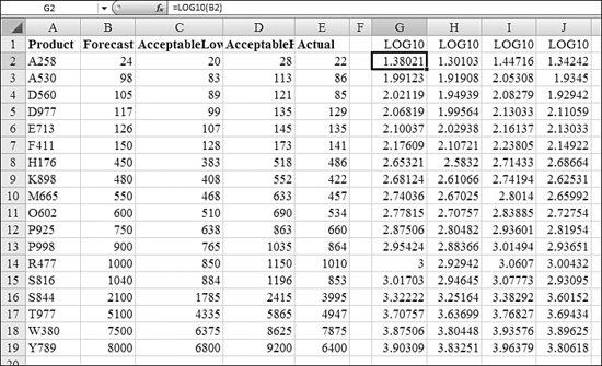
10^1 is 10. 10^2 is 100. The number in Cell B3 is 98. This logarithm is going to be between 1 and 2, and probably much closer to 2. The formula in Cell G3 reveals that if 10 is raised to the 1.99126th power, you get 198.

As another example, 10^2 is 100, and 10^3 is 1,000. Cell B17 contains 5,100. The logarithm for 5,100 is somewhere between 2 and 3. The formula in Cell G17, =LOG10(B17), shows that 10^3.707 results in 5,100.

Excel offers four functions for dealing with logarithms. LOG10 calculates the logarithms based on raising 10 to a certain power. LOG can calculate the logarithm for any base. LN and EXP deal with a special logarithm.

Syntax: LOG10(number)

The LOG10 function returns the base-10 logarithm of a number. The argument number is the positive real number for which you want the base-10 logarithm.

Using LOG to Calculate Logarithms for Any Base

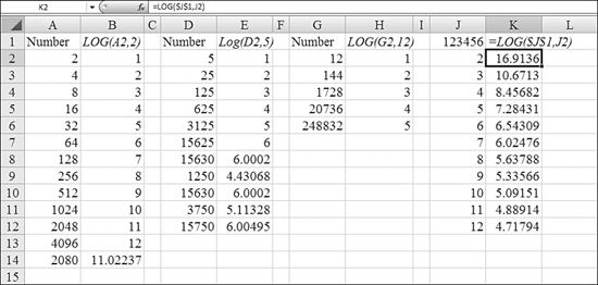
Excel makes it simple to calculate the logarithm for any base, using the LOG function. Cell B2 of Figure 27.14 contains the formula =LOG(A2,2) to express the number in Column A as a base-2 logarithm. Cell E2 contains the formula =LOG(E2,2) to express the number in Column E as a base-5 logarithm.

Figure 27.14. The LOG function can calculate a logarithm with any base.

Syntax: LOG(number,base)

The LOG function returns the logarithm of a number to the specified base. It takes the following arguments:

• number—This is the positive real number for which you want the logarithm.
• base—This is the base of the logarithm. If base is omitted, it is assumed to be 10.

Using LN and EXP to Calculate Natural Logarithms

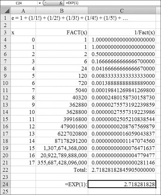
In science, only two logarithms are used frequently. The first is the base-10 logarithm discussed previously. The second is a natural logarithm where numbers are expressed as a power of the number e. e is a special number. You can calculate e by adding up all the numbers in the series of 1 + [1 / (1!)] + [1 / (2!)] + [1 / (3!)] + [1 / (4!)] + [1(5!)] + [1 / (7!)] + [1(8!)] + [1 / (9!)] + [1 / (10!)] + ....

Luckily, 10! is 3.7 million, so 1 / (10!) is a very small number: 0.000000275573. After about 1 / (17!), the numbers are small enough that they are beyond Excel’s 15-digit precision.

This infinite series converges toward a number around 2.718281. This number is known as the transcendental number and is abbreviated as e. Logarithms for base e are known as natural logarithms. You can calculate e in Excel by using a range such as the one shown in A4:C22 in Figure 27.15, or you can simply use =EXP(1), as shown in Cell C24.

Figure 27.15. The calculation of e is fairly complex, as shown in A4:C22. Instead, you can use =EXP(1).

Natural logarithms are very popular in science because anything with a constant rate of growth follows a curve described by natural logarithms. Radioactive isotopes, for example, decay along a curve described by natural logarithms.

While common logarithms with base 10 are called logs, natural logarithms with base e are written as ln (often pronounced lon). You calculate natural logarithms by using the LN function.

Syntax: LN(number)

The LN function returns the natural logarithm of a number. Natural logarithms are based on the constant e (that is, 2.71828182845904). The argument number is the positive real number for which you want a natural logarithm.

With common logarithms, you can easily convert the logarithm back to the original number by using =10^x. However, it is fairly difficult to write 2.71828182845904^x. Therefore, Excel provides the function EXP to raise e to any power.

Syntax: EXP(number)

The EXP function returns e raised to the power of number. The constant e equals 2.71828182845904, the base of the natural logarithm. The argument number is the exponent applied to the base e.

To calculate powers of other bases, you use the exponentiation operator (^). EXP is the inverse of LN, the natural logarithm of number.

To convert the logarithms in Column B in Figure 27.16, you use EXP(B2), as shown in Column C.

Figure 27.16. To reverse the LN function, you use EXP.

The decay of radioactive isotopes follows a natural logarithmic curve. The basic formula is as follows:

Number of atoms after time T = Original number of atoms × e^(T × Constant).

For Radium 226, the constant is –0.000436. The table in Figure 27.17 shows how to raise e to a certain power by using a table of years. You can see that about half the original sample will have decayed after 1,500 years!

Figure 27.17. For constant growth or decay problems, you can use EXP to raise e to a power.

Working with Imaginary Numbers

Multiply the number 2 by itself: =2^2 is 4. The square root of 4 is 2. Multiply the number –2 by itself: =-2^2 is also 4. Excel says =SQRT(4) is 2, but clearly it could also be -2 as well.

So, what is the square root of –4? There is no real number that produces –4 when multiplied by itself. Excel says that =SQRT(-4) is #NUM!.

To deal with theoretical numbers where the square root is a negative number, mathematicians invented the concept of the imaginary number, i. This number is the square root of –1. At first, no one was sure if this was relevant, so these numbers were given the name imaginary numbers. Since their invention, imaginary numbers have been discovered to have real-world applications. They are used extensively in the physics of electrical circuits. The name imaginary continues to stick.

In the parlance of imaginary numbers, the square root of –4 is 2i.

Often, the answer to a problem appears as an expression such as a + b × i. In this case, both a and b are real numbers. This expression is a complex number. You can plot complex numbers on a coordinate graph (plotting a along the x-axis and b along the y axis) and do trigonometry with imaginary numbers.

Excel offers nine functions that deal with imaginary, or complex, numbers: COMPLEX, IMREAL, IMAGINARY, IMSUM, IMPRODUCT, IMDIV, IMABS, IMARGUMENT, and IMCONJUGATE.

Using COMPLEX to Convert a and b into a Complex Number

It is hard to deal with complex numbers in Excel because they are basically text. Think about how you can store 5 + 2i in a cell; it would be difficult to do.

You can easily create a large range of complex numbers in the form a + bi if you have ranges of values for a and b. In Figure 27.18, pairs of a and b values are stored in the first two columns of a worksheet. The COMPLEX function in Column C converts these numbers to complex numbers.

Figure 27.18. The COMPLEX function builds text results in Column C. The eight IM functions can do math on these text values.

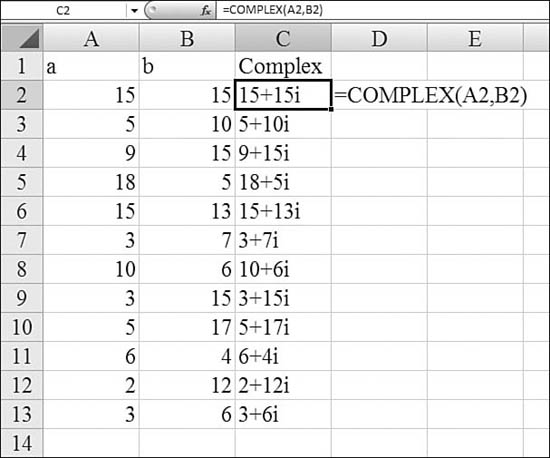
Syntax: COMPLEX(real_num,i_num,suffix)

The COMPLEX function converts real and imaginary coefficients into a complex number in the form x + yi or x + yj. This function takes the following arguments:

• real_num—This is the real coefficient of the complex number.
• i_num—This is the imaginary coefficient of the complex number.
• suffix—This is the suffix for the imaginary component of the complex number. If omitted, suffix is assumed to be i.

If real_num is nonnumeric, COMPLEX returns a #VALUE! error. If i_num is nonnumeric, COMPLEX returns a #VALUE! error. If suffix is neither i nor j, COMPLEX returns a #VALUE! error.

Using IMREAL and IMAGINARY to Break Apart Complex Numbers

Complex numbers are in the form a + bi, where i is the imaginary square root of –1. Excel stores all complex numbers as text. If you use any of the IM functions to generate new complex numbers, you can extract the numbers a and b by using IMREAL and IMAGINARY.

In Figure 27.19, Column A contains a range of complex numbers. The formulas in Column B extract the real number portion of the complex number. The formulas in Column C extract the value that is multiplied by i in the complex number.

Figure 27.19. IMREAL and IMAGINARY break a complex number expression in the form a + bi into the numbers for a and b.

Syntax: IMREAL(inumber)

The IMREAL function returns the real coefficient of a complex number in x + yi or x + yj text format. The argument inumber is a complex number for which you want the real coefficient.

If inumber is not in the form x + yi or x + yj, IMREAL returns a #NUM! error.

Syntax: IMAGINARY(inumber)

The IMAGINARY function returns the imaginary coefficient of a complex number in x + yi or x + yj text format. The argument inumber is a complex number for which you want the imaginary coefficient.

If inumber is not in the form x + yi or x + yj, IMAGINARY returns a #NUM! error.

Using IMSUM to Add Complex Numbers

Figure 27.20 shows two columns of complex numbers. A complex number is in the form a + bi. Both a and b are real numbers. The letter i is the imaginary square root of –1.

Figure 27.20. Even though all the complex numbers in Columns A and B are text, the IMSUM function adds them with ease.

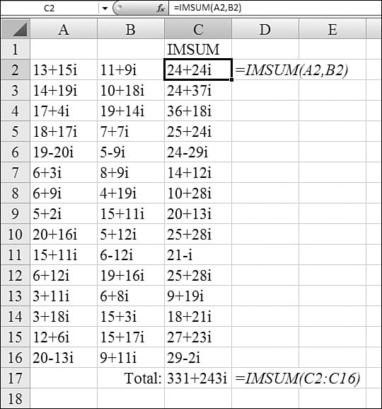
Note that all of the “numbers” stored in Columns A and B are stored as text.

To add (a + bi) + (c + di), you use the formula (a + b) + (c + d) i. You use IMSUM to calculate this.

Syntax: IMSUM(inumber1,inumber2,...)

The IMSUM function returns the sum of two or more complex numbers in x + yi or x + yj text format. The arguments inumber1,inumber2,... are 1 to 255 complex numbers to add.

If any argument is not in the form x + yi or x + yj, IMSUM returns a #NUM! error.

Using IMSUB, IMPRODUCT, and IMDIV to Perform Basic Math on Complex Numbers

As with the IMSUM function, there are similar rules for subtracting, multiplying, and dividing complex numbers. These are numbers stored as text in the form a + bi, where the constant i is an imaginary number representing the square root of –1. These are the rules for the IMSUB, IMPRODUCT, and IMDIV functions:

• To subtract complex numbers, you use IMSUB. The formula for (a + bi) – (c + di) is (a – c) + (b – d) i.
• To multiply complex numbers, you use IMPRODUCT. The formula for (a + bi) × (c + di) is (ac – bd) + (ad + bc) i.
• To divide complex numbers, you use IMDIV. The formula for (a + bi) / (c + di) is [(ac + bd) + (bc – ad) i] / (c^2 + d^2).

Figure 27.21 shows the results of the basic math functions for complex numbers.

Figure 27.21. You can perform basic math with complex numbers.

Syntax: IMSUB(inumber1,inumber2)

The IMSUB function returns the difference between two complex numbers in x + yi or x + yj text format. This function takes the following arguments:

• inumber1—This is the complex number from which to subtract inumber2.
• inumber2—This is the complex number to subtract from inumber1.

If either number is not in the form x + yi or x + yj, IMSUB returns a #NUM! error.

Syntax: IMPRODUCT(inumber1,inumber2,...)

The IMPRODUCT function returns the product of 2 to 255 complex numbers in x + yi or x + yj text format. The arguments inumber1, inumber2,... are 1 to 255 complex numbers to multiply.

If inumber1 or inumber2 is not in the form x + yi or x + yj, IMPRODUCT returns a #NUM! error.

Syntax: IMDIV(inumber1,inumber2)

The IMDIV function returns the quotient of two complex numbers in x + yi or x + yj text format. This function takes the following arguments:

• inumber1—This is the complex numerator or dividend.
• inumber2—This is the complex denominator or divisor.

If inumber1 or inumber2 is not in the form x + yi or x + yj, IMDIV returns a #NUM! error.

Using IMABS to Find the Distance from the Origin to a Complex Number

A complex number is in the form a + bi, where i is an imaginary number representing the square root of –1. To plot complex numbers on a Cartesian grid, you use a for the x-axis and b for the y-axis.

The IMABS function calculates the distance from the (0, 0) origin in the grid. If you have a complex number in the form a + bi, the formula for an absolute value is =SQRT(a^2+b^2). This results in a real number.

Syntax: IMABS(inumber)

The IMABS function returns the absolute value (modulus) of a complex number in x + yi or x + yj text format. The argument inumber is a complex number for which you want the absolute value.

If inumber is not in the form x + yi or x + yj, IMABS returns a #NUM! error.

Figure 27.22 shows IMABS functions for several complex numbers. Note that the result of IMABS(a+bi) is equal to IMABS(b+ai).

Figure 27.22. Taking the absolute value of a complex number results in a real number.

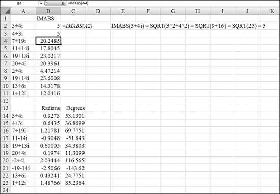
Using IMARGUMENT to Calculate the Angle to a Complex Number

A complex number is in the form a + bi, where i is an imaginary number representing the square root of –1. To plot complex numbers on a Cartesian grid, you use a for the x-axis and b for the y-axis.

The angle to a complex number assumes that the x-axis is 0 and rotates counter-clockwise. To find the angle, in radians, to any complex number plotted on a grid, you use IMARGUMENT.

B14:B23 in Figure 27.22 shows the angle for several complex numbers.

Syntax: IMARGUMENT(inumber)

The IMARGUMENT function returns the angle (θ) for an imaginary number. inumber is a complex number for which you want to calculate theta.

If inumber is not in the form x + yi or x + yj, IMARGUMENT returns a #NUM! error.

Using IMCONJUGATE to Reverse the Sign of an Imaginary Component

A complex number is in the form a + bi, where i is an imaginary number representing the square root of –1. To plot complex numbers on a Cartesian grid, you use a for the x-axis and b for the y-axis.

The IMCONJUGATE function creates a mirror image of a point, flipped across the x-axis. Put another way, the function changes the sign of the imaginary component. For example, 10 + 3i becomes 10 – 3i, and 10 – 3i becomes 10 + 3i.

Syntax: IMCONJUGATE(inumber)

The IMCONJUGATE function returns the complex conjugate of a complex number in x + yi or x + yj text format. The argument inumber is a complex number for which you want the conjugate.

If inumber is not in the form x + yi or x + yj, IMCONJUGATE returns a #NUM! error.

Figure 27.23 shows the results of several IMCONJUGATE formulas.

Figure 27.23. You can reverse the sign of the imaginary component of a complex number with IMCONJUGATE.

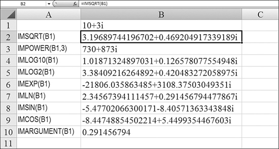
Calculating Powers, Logarithms, and Trigonometry Functions with Complex Numbers

The remaining eight IM functions calculate powers, exponents, logs, and trig functions from complex numbers:

• IMSQRT—This function calculates the square root of a complex number.
• IMPOWER—This function raises a complex number to a certain power.
• IMLOG10—This function calculates the base-10 logarithm or common logarithm of a complex number.
• IMLOG2—This function calculates the base-2 logarithm of a complex number.
• IMEXP—This function raises the constant e to a complex number. For more information, see the information on EXP, earlier in this chapter.
• IMLN—This function calculates the natural log of a complex number.
• IMSIN—This function calculates the sine of a complex number.
• IMCOS—This function calculates the cosine of a complex number.

Figure 27.24 shows the results of these functions for a complex number.

Figure 27.24. These functions calculate powers, logs, and trig functions, using text-based complex numbers.

Solving Simultaneous Linear Equations with Matrix Functions

You can use the Solver add-in to solve simultaneous equations, but Excel also offers three matrix functions that you can use to solve them. While the math involved in this is beyond the scope of this book, the steps in producing an answer are fairly straightforward.

The following is a problem taken from a math textbook in the Han Dynasty. The solution can easily be derived by using matrix functions in Excel.

There are three types of grain. Three bundles of the first, two of the second, and one of the third make 39 bushels. Two of the first, three of the second, and one of the third make 34 bushels. One of the first, two of the second, and three of the third make 26 bushels. How many bushels are in the bundles of each type of grain? To solve this problem, you follow these steps:

1. Convert the problem’s words into algebraic equations. Assuming that the first type of grain is a, the second is b, and the third is c, you have these three equations:
   3a + 2b + 1c = 39
   2a + 3b + 1c = 34
   1a + 2b + 3c = 26
2. In Excel, set up three columns with headings a, b, and c. In the three rows below these columns, enter the coefficients from each equation. For example, the first row would contain 3, 2, and 1. The second row would contain 2, 3, and 1. The third row would contain 1, 2, and 3. In Figure 27.25, the range C5:E7 contains the matrix of coefficients.

   Figure 27.25. Amazingly, Excel can solve simultaneous equations by using a pair of matrix functions.

   

3. In another range, enter a matrix of the answers for each equation. This range should be one column wide by three rows tall. The cells should contain 39, 34, and 26. In Figure 27.25, this range is in G5:G7.
4. Select a new range that is the same size as the range in step 2. This range will hold an intermediate step with the inverse matrix. In the new range, type the formula =MINVERSE(C5:E7). Do not press Enter. Instead, hold down Ctrl+Shift while you press Enter. This key combination tells Excel to calculate an array and enter the results in all the selected cells. (See range C10:E12 in Figure 27.25.)

   The inverse of an array is an array that, when multiplied by the original array, produces a new array with 1s along the diagonal and 0s everywhere else. In Figure 27.25, the range C15:E17 contains the array formula =MMULT(C5:E7,C10:E12). As you can see in Figure 27.25, the result of the MMULT operation is indeed a matrix with a 1 along the diagonal and 0s everywhere else.

5. Select a range that is three cells high and one column wide. In this column, enter a MMULT function that multiplies the MINVERSE array from step 4 by the answers in step 3. In Figure 27.25, the formula in I5:I7 is =MMULT(C10:E12,G5:G7). Again, you must select all three cells before entering this formula, and you must hold down Ctrl+Shift+Enter to enter the formula. The results in Cells I5, I6, and I7 stand for the values of a, b, and c, respectively.
6. To make sure that everything worked, set up test formulas in column K. For example, the test formula in K5 checks to see if 3a+2b+c equals 39.

This entire process is fairly amazing. All the formulas are live formulas. If you change one of the input variables in any of the ranges, all the matrix functions instantly recalculate to solve the three simultaneous equations.

Syntax: MINVERSE(array)

The MINVERSE function returns the inverse matrix for the matrix stored in an array. The argument array is a numeric array with an equal number of rows and columns. array can be given as a cell range, such as A1:C3; as an array constant, such as {1,2,3;4,5,6;7,8,9}; or as a name for either of these.

If any cells in array are empty or contain text, MINVERSE returns a #VALUE! error. MINVERSE also returns a #VALUE! error if array does not have an equal number of rows and columns.

Formulas that return arrays must be entered as array formulas.

Inverse matrices, like determinants, are generally used for solving systems of mathematical equations that involve several variables. The product of a matrix and its inverse is the identity matrix—the square array in which the diagonal values equal 1 and all other values equal 0.

As an example of how a two-row, two-column matrix is calculated, suppose that the range A1:B2 contains the letters a, b, c, and d, which represent any four numbers. Table 27.5 shows the inverse of the matrix A1:B2.

Table 27.5. Inverse of the Matrix Shown in A1:B2 (see Figure 27.26)

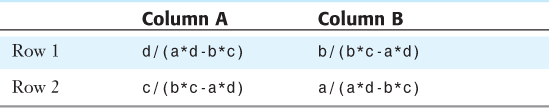
Figure 27.26. Range A6:B7 contains the MINVERSE of the original array. When you multiply an array and its MINVERSE array, the resulting array in A10:B11 contains 1s along the diagonal.

MINVERSE is calculated to an accuracy of approximately 16 digits, which may lead to a small numeric error when the cancellation is not complete. Thus, when you use MMULT on this array with the original array, you might find 0.00000000000001 instead of 0 in some cells.

Some square matrices cannot be inverted and return a #NUM! error with MINVERSE. The determinant for a noninvertable matrix is 0.

The MMULT function multiplies two arrays. The basic logic is that the top-left cell of the resulting array is the sum of multiplying the first row of Array 1 by the first column of Array 2. Figure 27.27 shows the rest of the rules for a 2 × 2 matrix.

Figure 27.27. The MMULT function performs matrix multiplication.

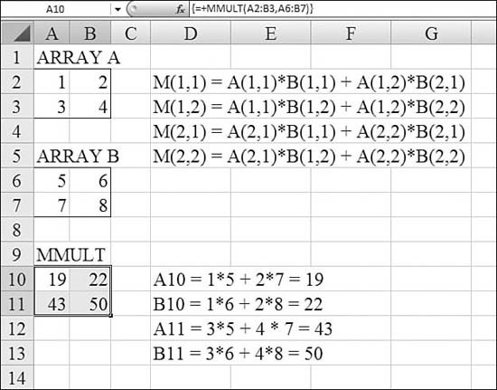
Syntax: MMULT(array1,array2)

The MMULT function returns the matrix product of two arrays. The result is an array with the same number of rows as array1 and the same number of columns as array2.

The arguments array1 and array2 are the arrays you want to multiply. The number of columns in array1 must be the same as the number of rows in array2, and both arrays must contain only numbers. array1 and array2 can be given as cell ranges, array constants, or references. If any cells are empty or contain text, or if the number of columns in array1 is different from the number of rows in array2, MMULT returns a #VALUE! error.

In Figure 27.27, A2:B3 contains Array A. A6:B7 contains Array B. The result of the MMULT formula, Array M, is in A10:B11. The rules for the calculation of each cell in M are shown in D2:D5. The actual formulas are shown in D10:D13.

Using MDETERM to Determine Whether a Simultaneous Equation Has a Solution

If your matrix of simultaneous equations is square, Excel can calculate a determinant of the array by using MDETERM. The determinant returns a single number, so this function does not need to be entered as an array. If the determinant of an array is nonzero, the simultaneous equation has a solution.

Figure 27.28 shows the calculation for the determinant of a 2 × 2 matrix.

Figure 27.28. MDETERM returns the determinant of any square array. Determinants that are nonzero indicate that the simultaneous equations have a solution.

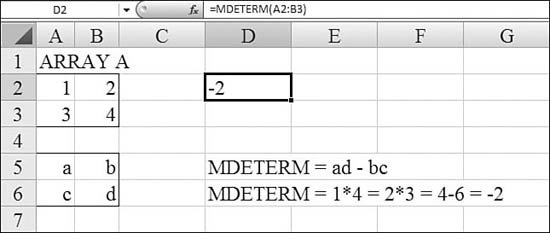
Syntax: MDETERM(array)

The MDETERM function returns the matrix determinant of an array. The argument array is a numeric array with an equal number of rows and columns. array can be given as a cell range, such as A1:C3; as an array constant, such as {1,2,3;4,5,6;7,8,9}; or as a name to either of these. If any cells in array are empty or contain text, MDETERM returns a #VALUE! error. MDETERM also returns #VALUE! if array does not have an equal number of rows and columns.

The matrix determinant is a number derived from the values in array. For a three-row, three-column array, A1:C3, the determinant is defined as follows:

MDETERM(A1:C3) = A1*(B2*C3-B3*C2) + A2*(B3*C1-B1*C3) + A3*(B1*C2-B2*C1)

Matrix determinants are generally used for solving systems of mathematical equations that involve several variables.

MDETERM is calculated with an accuracy of approximately 16 digits, which may lead to a small numeric error when the calculation is not complete. For example, the determinant of a singular matrix may differ from zero by 1E – 16.

Figure 27.28 shows a MDETERM calculation for a 2×2 array.

Using SERIESSUM to Approximate a Function with a Power Series

There are situations in mathematics in which a value can be approximated by summing many factors in a series. If the series gets progressively smaller (for example, ½, , ¼, , , ) the numbers eventually become smaller than Excel’s 15-digit significance limit. This is referred to as a power series. In a power series, the exponent of each term is progressively changed. An example of a power series is =a₁x^1 + a₂x^3 + a₃x^5 + a₄x^7 + a₅x^9.

Figure 27.29 shows a very long, complex calculation. The coefficients in Column D are found by dividing factorials of even number digits into the number 1 and then multiplying every other value by –1. The value of x is 60 degrees, or PI() / 3. The exponents shown in Column E increase from 0 to 16 by 2s. In Column F, you raise X to the power in Column E. In Column G, you multiply Column D by Column F. Finally, you add up all the values in Column G to arrive at 0.5, which is a really good approximation of the cosine of 60 degrees.

Figure 27.29. The SERIESSUM function can calculate a power series, given a value X, a pattern for the exponents, and a list of coefficients.

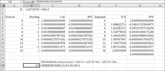
This example is rather trivial because Excel actually offers a COS function. However, other functions use a power series to approximate a function. For example, one SERIESSUM function in B17 replaces all the calculations in Columns E, F, and G. The function needs the list of coefficients in Column D. In fact, the number of coefficients tells Excel how far to extend the series.

Syntax: SERIESSUM(x,n,m,coefficients)

The SERIESSUM function returns the sum of a power series. Many functions can be approximated by a power series expansion. This function takes the following arguments:

• x—This is the input value to the power series.
• n—This is the initial power to which you want to raise x.
• m—This is the step by which to increase n for each term in the series.
• coefficients—This is a set of coefficients by which each successive power of x is multiplied. The number of values in coefficients determines the number of terms in the power series. For example, if there are three values in coefficients, there will be three terms in the power series.

If any argument is nonnumeric, SERIESSUM returns a #VALUE! error.

Using SQRTPI to Find the Square Root of a Number Multiplied by Pi

The SQRTPI function multiplies a number by Π and then takes the square root of the result. Because my exposure to Π is usually based on figuring out which pizza is the best deal, I’ve never had the occasion to multiply a number by Π and take the square root of the result. However, if your job requires you to take the square root of a number multiplied by Π, the SQRTPI function is just waiting for you to use it.

Syntax: SQRTPI(number)

The SQRTPI function returns the square root of (number × Π). The argument number is the number by which Π is multiplied. If number is less than 0, SQRTPI returns a #NUM! error.

=SQRTPI(5) calculates 5*PI() as 15.7 and then takes the square root of 15.7, to return 3.96.

Using SUMPRODUCT to Sum Based on Multiple Conditions

The use of SUMPRODUCT will be dropping dramatically in Excel 2007. Until this point, SUMPRODUCT was one of the favorite methods for solving a particular limitation with SUMIF. However, since Microsoft added the SUMIFS function to Excel 2007, there will be less need for SUMPRODUCT.

In case you need to share your workbooks with people using prior versions of Excel, you can work through this example to solve the problem of conditionally summing a range based on two conditions. Say that you are starting with the data in column A:C of Figure 27.30. This simple dataset has fields for region, product, and sales.

Figure 27.30. The rather long and winding calculations in E2:G18 answer how many units meet two conditions. A single formula in B23 replaces all these steps.

The SUMIF command could easily add up all the sales that occurred in the east: =SUMIF(A2:A17,"East",C2:C17). But there is no way to use SUMIF to find the sum of all records that are in the east and for Product A. Using SUMPRODUCT to solve this problem requires you to think about a couple virtual arrays. I’ve actually entered these arrays as intermediate steps in Figure 27.30 so that you can picture them:

• In Column E, the formula tests whether the cell in Column A is equal to East.
• In Column F, the formula tests whether the cell in Column B is equal to A.
• Column G contains an interesting formula. Cell G2 multiplies the sales in Cell C2 by the TRUE/FALSE value in Cell E2 and then multiplies that by the TRUE/FALSE value in Cell G2. In Excel’s treatment of TRUE/FALSE values, a TRUE is calculated as a 1, and a FALSE is calculated as a 0. Thus, in Cell G2, the 8 × TRUE × TRUE is like multiplying 8 × 1 × 1, which results in 8.
• If either cell in Column E or Column F is FALSE, Excel treats the value as a zero. Because zero times anything is zero, the result in Column G shows up as zero if the corresponding value in either Column E or Column F is FALSE.
• In Cell G18, a SUM function totals the products from Column G in order to answer how many sales of Product A were made in the east.

The SUMPRODUCT function does all the steps from Columns E, F, and G in a single function, as shown in Cell B23 in Figure 27.30.

Syntax: SUMPRODUCT(array1,array2,array3,...)

The SUMPRODUCT function multiplies corresponding components in the given arrays and returns the sum of those products. The arguments array1, array2, array3,... are 2 to 255 arrays whose components you want to multiply and then add together.

The array arguments must have the same dimensions. If they do not, SUMPRODUCT returns a #VALUE! error. SUMPRODUCT treats array entries that are not numeric as if they were zeros.

To solve a problem that has multiple conditions, you have to create three virtual arrays in the function arguments. Here’s how you do it:

1. Make the first array the sales in C2:C17.
2. Make the second array a test to see if A is equal to East. This would be (A2:A17="East").
3. Make the third array a test to see if B is equal to A. This would be (B2:B17="A").
4. Multiply these three arrays to get the formula =SUMPRODUCT((C2:C17)*(A2:A17="East")*(B2:B17="A")). This provides a result of 26, just as in the previous example.
5. Make the function from step 4 more generic. In Figure 27.30, a summary table in A19:C22 has the headings East, Central, West, A, and B. The formula in B20 is =SUMPRODUCT(($C$2:$C$17)*($A$2:$A$17=$A20)*($B$2:$B$17=B$19)). This formula adds dollar signs so that the formula can be easily copied. It also replaces "East" with $A20 and "A" with B$19.
6. Copy this formula to the rest of the table. You now have an efficient conditional total that sums records based on two criteria.

Examples of Engineering Functions

There are not many true engineering functions in Excel. You will notice that I reclassified most of the IM functions into the previous section on imaginary numbers. All the BIN2, DEC2, HEX2, and OCT2 functions are, at best, interesting to software engineers.

The CONVERT function is interesting to everyone and is truly the one engineering function that could have been shown in Chapter 23, “Using Everyday Functions: Math, Date and Time, and Text Functions.”

So there are just a handful of true engineering functions: The various BESSEL functions, ERF, DELTA, and the GESTEP functions are of use exclusively to engineers.

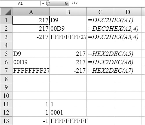
Converting from Decimal to Hexadecimal and Back

A long time ago, I held a summer internship writing COBOL programs for a company. Whenever one of my programs crashed in the middle of the night, I was supposed to show up and read through a hexadecimal printout of the computer memory to figure out what went wrong.

In the hexadecimal numbering system, there are 16 digits. The digits, in order, are 0, 1, 2, 3, 4, 5, 6, 7, 8, 9, A, B, C, D, E, and F. The number that you and I know as 10 would be written as A in hexadecimal. The number 15 would be written as F in hexadecimal. After F comes the hexadecimal number 10, which is equivalent to 16 in decimal.

Hexadecimal numbers can get rather large. For example, the hex number C2 means 12 × 16 + 2 (remember that C is equivalent to a decimal 12). The hex number 1111 means 1 × 16^3 + 1 × 16^2 + 1 × 16 + 1, or 4,369.

There are actually calculators that let you add a number such as A52B with C2D4 to come up with the answer 167FF.

In Excel, you can easily convert numbers in the base-10 system to hexadecimal by using DEC2HEX. Similarly, you can convert hex numbers to a base-10 numbering system by using HEX2DEC.

Syntax: DEC2HEX(number,places)

The DEC2HEX function converts a decimal number to hexadecimal. This function takes the following arguments:

• number—This is the decimal integer you want to convert. If number is negative, places is ignored, and DEC2HEX returns a 10-character (that is, 40-bit) hexadecimal number in which the most significant bit is the sign bit. The remaining 39 bits are magnitude bits. Negative numbers are represented using two’s-complement notation.
• places—This is the number of characters to use. If places is omitted, DEC2HEX uses the minimum number of characters necessary. places is useful for padding the return value with leading 0s.

If number is less than –549,755,813,888 or if number is greater than 549,755,813,887, DEC2HEX returns a #NUM! error. If number is nonnumeric, DEC2HEX returns a #VALUE! error. If DEC2HEX requires more than places characters, it returns a #NUM! error.

If places is not an integer, it is truncated. If places is nonnumeric, DEC2HEX returns a #VALUE! error. If places is negative, DEC2HEX returns a #NUM! error.

Syntax: HEX2DEC(number)

The HEX2DEC function converts a hexadecimal number to decimal. The argument number is the hexadecimal number you want to convert. number cannot contain more than 10 characters (that is, 40 bits). The most significant bit of number is the sign bit. The remaining 39 bits are magnitude bits. Negative numbers are represented using two’s-complement notation.

If number is not a valid hexadecimal number, HEX2DEC returns a #NUM! error.

Figure 27.31 shows a conversion from decimal to hexadecimal and back. Note that Cell B2 uses the places argument to specify that leading zeros should be added to generate a number that is 4 digits long.

Figure 27.31. Converting from decimal to hexadecimal and back.

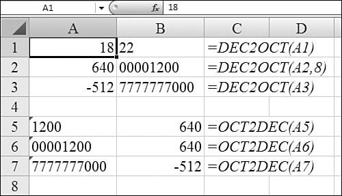
Converting from Decimal to Octal and Back

The octal numbering system is a base-8 numbering system. In this system, there are only eight digits, from 0 through 7. The decimal number 8 is represented in octal as 10.

Each numeric place in an octal number represents an additional power of 8. The octal number 1111 represents 1 × 8^3 + 1 × 8^2 + 1^8 + 1, or 512 + 64 + 8 + 1, or 585 in decimal.

You use DEC2OCT to convert from decimal to octal and OCT2DEC to convert from octal to decimal.

Syntax: DEC2OCT(number,places)

The DEC2OCT function converts a decimal number to octal. This function takes the following arguments:

• number—This is the decimal integer you want to convert. If number is negative, places is ignored, and DEC2OCT returns a 10-character (that is, 30-bit) octal number in which the most significant bit is the sign bit. The remaining 29 bits are magnitude bits. Negative numbers are represented using two’s-complement notation.
• places—This is the number of characters to use. If places is omitted, DEC2OCT uses the minimum number of characters necessary. places is useful for padding the return value with leading 0s.

If number is less than –536,870,912 or if number is greater than 536,870,911, DEC2OCT returns a #NUM! error. If number is nonnumeric, DEC2OCT returns a #VALUE! error. If DEC2OCT requires more than places characters, it returns a #NUM! error. If places is not an integer, it is truncated. If places is nonnumeric, DEC2OCT returns a #VALUE! error. If places is negative, DEC2OCT returns a #NUM! error.

Syntax: OCT2DEC(number)

The OCT2DEC function converts an octal number to decimal. The argument number is the octal number you want to convert. number cannot contain more than 10 octal characters (that is, 30 bits). The most significant bit of number is the sign bit. The remaining 29 bits are magnitude bits. Negative numbers are represented using two’s-complement notation.

If number is not a valid octal number, OCT2DEC returns a #NUM! error.

Figure 27.32 shows a conversion from decimal to octal and back.

Figure 27.32. The places argument in Cell B2 controls the leading zeroes.

Converting from Decimal to Binary and Back

Although hexadecimal and octal numbering systems are seldom encountered anymore, many people still encounter binary number systems. Binary number systems are the language of computers because every circuit has a state of either 1 (meaning that electricity is present) or 0 (meaning that electricity is not present). Thus, the binary number system has only 2 digits, 0 and 1:

• The rightmost digit in a binary number means 0 or 1.
• The next rightmost digit represents 2^1, or 2.
• The next digit represents 2^2, or 4.
• The next digit represents 2^3, or 8.
• The next digit represents 2^4, or 16.
• The next digit represents 2^5, or 32.
• The next digit represents 2^6, or 64.

For example, the binary number 1010101 means 64 + 16 + 4 + 1, or 85 in decimal. You use DEC2BIN to convert from decimal to binary and BIN2DEC to convert from binary to decimal. Note that DEC2BIN only works with the numbers 512 and lower.

Syntax: DEC2BIN(number,places)

The DEC2BIN function converts a decimal number to binary. This function takes the following arguments:

• number—This is the decimal integer you want to convert. If number is negative, places is ignored, and DEC2BIN returns a 10-character (that is, 10-bit) binary number in which the most significant bit is the sign bit. The remaining 9 bits are magnitude bits. Negative numbers are represented using two’s-complement notation.
• places—This is the number of characters to use. If places is omitted, DEC2BIN uses the minimum number of characters necessary. places is useful for padding the return value with leading 0s.

If number is less than –512 or if number is greater than 511, DEC2BIN returns a #NUM! error. If number is nonnumeric, DEC2BIN returns a #VALUE! error. If DEC2BIN requires more than places characters, it returns the #NUM! error. If places is not an integer, it is truncated. If places is nonnumeric, DEC2BIN returns a #VALUE! error. If places is negative, DEC2BIN returns a #NUM! error.

Syntax: BIN2DEC(number)

The BIN2DEC function converts a binary number to decimal. The argument number is the binary number you want to convert. number cannot contain more than 10 characters (that is, 10 bits). The most significant bit of number is the sign bit. The remaining 9 bits are magnitude bits. Negative numbers are represented using two’s-complement notation.

If number is not a valid binary number, or if number contains more than 10 characters (that is, 10 bits), BIN2DEC returns a #NUM! error.

The formulas in Figure 27.33 convert from decimal to binary and from binary to decimal.

Figure 27.33. Converting from decimal to binary and back.

Explaining the Two’s Complement for Negative Numbers

In all the previous examples, the hex, octal, and binary numbers look bizarre for negative numbers. This is a special notation called two’s complement. In Excel, we have to agree that a negative number occupies 10 characters. For example, Cell A1 in Figure 27.34 contains the number five in binary.

Figure 27.34. Negative numbers in two’s complement are initially unnerving, until you understand the steps for converting them.

If the leftmost bit is a 1, then the number is assumed to be negative, and Excel assumes that the number is in two’s-complement notation. There are two simple steps to convert a positive number to a negative number in two’s complement:

1. Change every 0 to a 1 and every 1 to a 0. This produces a number in one’s complement, as shown in Cell A2 in Figure 27.34.
2. Add 1 to the result from step 1 to convert to two’s complement, as shown in Cell A3 in Figure 27.34.

Note that the leftmost bit is always set to a 1 for a negative number. This prevents Excel from representing 512 in binary. The binary representation of 512—1000000000—has a 1 in the leftmost digit, so no numbers over 511 can be represented in binary in Excel.

Converting from negative to positive in two’s complement follows exactly the same method. Cell A13 in Figure 27.34 contains –5 in two’s complement. In Cell A14, you switch all the 0s and 1s. In Cell A15, you add 1 to produce the original result in binary.

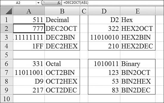
Converting from Binary to Hex to Octal and Back

Excel offers six additional functions that can convert directly from octal to hexadecimal to binary. The major limitation of these functions is that Excel can represent as binary only numbers up to 511 in decimal. This is a significant limitation; anything larger than 1FF in hex or larger than 777 in octal returns an error if you try to convert it to binary.

These are the additional conversion functions:

• BIN2HEX(number,places)—This converts a binary number to hexadecimal.
• BIN2OCT(number,places)—This converts a binary number to octal.
• HEX2BIN(number,places)—This converts a hexadecimal number to binary.
• HEX2OCT(number,places)—This converts a hexadecimal number to octal.
• OCT2BIN(number,places)—This converts an octal number to binary.
• OCT2HEX(number,places)—This converts an octal number to hexadecimal.

Figure 27.35 demonstrates these conversion functions.

Figure 27.35. You can convert between hex, octal, and binary by using these six functions.

Using CONVERT to Convert English to Metric

The CONVERT function is an incredibly versatile function. It can convert measures in the following areas:

• Weight and mass
• Distance
• Time
• Pressure
• Force
• Energy
• Power
• Magnetism
• Temperature
• Liquid measure

Syntax: CONVERT(number,from_unit,to_unit)

The CONVERT function converts a number from one measurement system to another. For example, CONVERT can translate a table of distances in miles to a table of distances in kilometers. This function takes the following arguments:

• number—This is the value in from_units to convert.
• from_unit—This is the units for number.
• to_unit—This is the units for the result.

Tables 27.6 through 27.15 list the text values that CONVERT accepts for from_unit and to_unit.

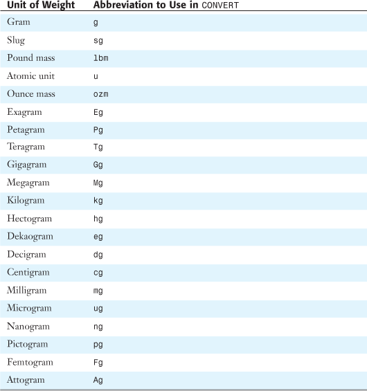
Table 27.6. Units of Weight and Mass

If the input data types are incorrect, CONVERT returns a #VALUE! error. If the unit does not exist, CONVERT returns an #N/A error.

If the unit does not support an abbreviated unit prefix, CONVERT returns an #N/A error.

If the units are in different groups, CONVERT returns an #N/A error.

The unit abbreviations to use in CONVERT are case-sensitive.

Table 27.6 shows conversions possible for weights.

Figure 27.36 shows a conversion of weights and masses.

Figure 27.36. This table converts between the mass units in the left column and the various units along the top row.

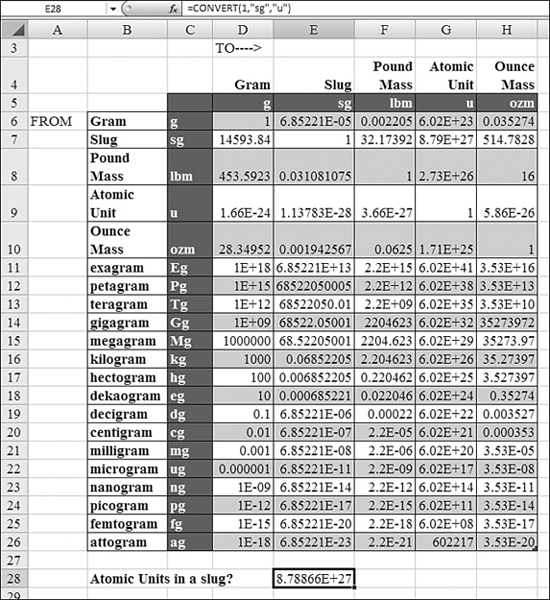
Table 27.7 shows conversion units for distance.

Table 27.7. Units of Distance

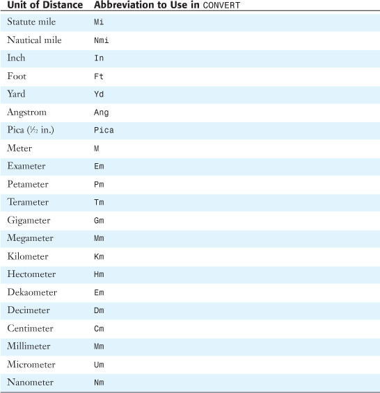
Figure 27.37 shows a conversion of distances.

Figure 27.37. This table converts between the distance units in the left column and the various units along the top row.

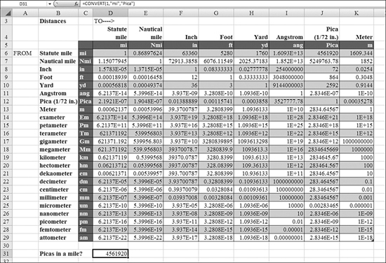
Table 27.8 shows conversion abbreviations for measures of time.

Table 27.8. Units of Time

Figure 27.38 shows a conversion of times.

Figure 27.38. This table converts between the time units in the left column and the various units along the top row.

Table 27.9 shows conversion values for units of pressure.

Table 27.9. Units of Pressure

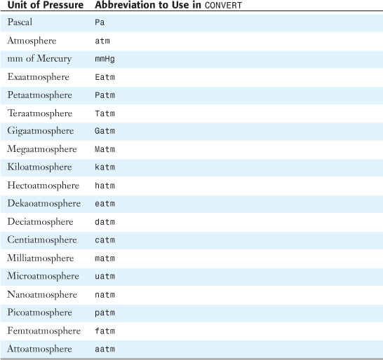
Figure 27.39 shows a conversion of pressures.

Figure 27.39. This table converts between the pressure units in the left column and the various units along the top row.

Table 27.10 shows conversion values for units of force.

Table 27.10. Units of Force

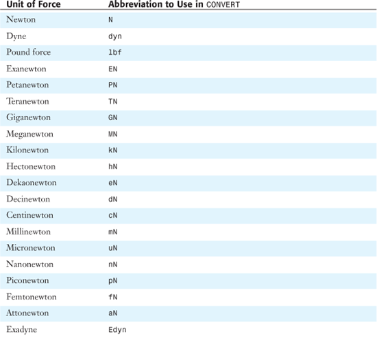
Figure 27.40 shows a conversion of forces.

Figure 27.40. This table converts between the force units in the left column and the various units along the top row.

Table 27.11 shows conversions available for energy.

Table 27.11. Units of Energy^[*]

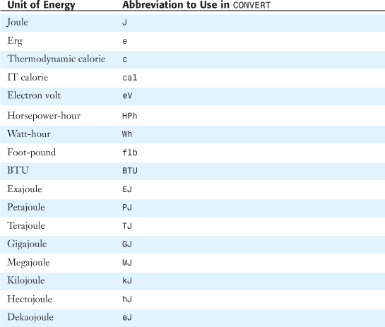
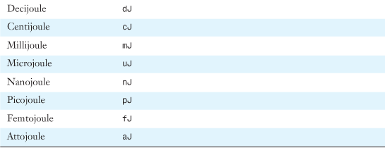
^[*] This table shows the complete metric prefixes for joules. Similar metric prefixes can also be applied to ergs, thermodynamic calories, IT calories, electron volts, and Watt-hours. This adds 80 additional measurements available in the CONVERT function for Energy.

Figure 27.41 shows a conversion of energies.

Figure 27.41. This table converts between the energy units in the left column and the various units along the top row.

Table 27.12 shows conversions available for power.

Table 27.12. Units of Power

Figure 27.42 shows a conversion of powers.

Figure 27.42. This table converts between the power units in the left column and the various units along the top row.

Table 27.13 shows conversions available for units of magnetism.

Table 27.13. Units of Magnetism

Figure 27.43 shows a conversion of magnetisms.

Figure 27.43. This table converts between the magnetism units in the left column and the various units along the top row.

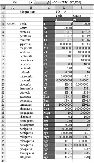
Table 27.14 shows conversion factors available for temperature systems.

Table 27.14. Units of Temperature

Figure 27.44 shows a conversion of temperature systems.

Figure 27.44. This table converts between the temperature scales in the left column and the various scales along the top row.

Table 27.15 shows conversion units available for liquid measurements.

Table 27.15. Units of Liquid Measure

Figure 27.45 shows a conversion of liquid measures.

Figure 27.45. This table converts between the liquid measurement units in the left column and the various units along the top row.

Using DELTA or GESTEP to Filter a Set of Values

The functions DELTA and GESTEP are left over from a long-ago era. In the SUMPRODUCT function, you can see that Excel can now evaluate TRUE*100 as 100 and FALSE*100 as 0. In early spreadsheet programs, you needed to explicitly convert TRUE to 1 and FALSE to 0. These two functions explicitly return 1 when a condition is true and 0 when a condition is false, allowing you to multiply the original number by the function in order to get conditional sums.

DELTA tests whether two values are equal. GESTEP tests whether a value is greater than or equal to a threshold value.

Syntax: DELTA(number1,number2)

The DELTA function tests whether two values are equal. It returns 1 if number1 equals number2; it returns 0 otherwise. You use this function to filter a set of values. For example, by summing several DELTA functions, you can calculate the count of equal pairs. This function is also known as the Kronecker Delta function. This function takes the following arguments:

• number1—This is the first number.
• number2—This is the second number. If omitted, number2 is assumed to be 0.

If either number1 or number2 is nonnumeric, DELTA returns a #VALUE! error.

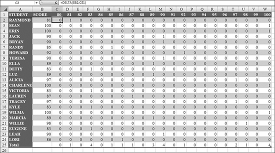
Figure 27.46 shows a list of students and their test scores in Columns A and B. A large matrix of DELTA functions in C:W counts how many students achieved each score. Excel has many newer, better functions, such as COUNTIF, that can also achieve this result.

Figure 27.46. The DELTA functions in C2:W24 check whether the score in Column B is the same as the score in Row 1. Totals in row 25 complete the analysis.

Syntax: GESTEP(number,step)

The GESTEP function returns 1 if number is greater than or equal to step; it returns 0 otherwise. You use this function to filter a set of values. For example, by summing several GESTEP functions, you can calculate the count of values that exceed a threshold. This function takes the following arguments:

• number—This is the value to test against step.
• step—This is the threshold value. If you omit a value for step, GESTEP uses 0.

If any argument is nonnumeric, GESTEP returns a #VALUE! error.

Using ERF and ERFC to Calculate the Error Function and Its Complement

An error function is designed to make it easier to represent integrals in the form x^n × e (–ax^2) dx. All such integrals can be written in terms of the integral e^(–u^2) du. If you integrate this from 0 to infinity, it converges to SQRT(PI)/2. The ERF function, then, is defined so that ERF converges to 1 at infinity.

The ERF function is ERF(x) = 2/SQRT(PI()) times the integral of e^(-u^2)du integrated from 0 to x. The result of ERF is a value between 0 and 1.

Contrary to what Excel Help says, there are two syntax options available in Excel for ERF:

• ERF(x)—The common use of ERF is with a single argument. In this case, the function returns the ERF function. In the preceding formula, the integral is evaluated from 0 to x. For example, ERF(0.1) is 0.112463.
• ERF(lower_limit,upper_limit)—The second syntax for ERF provides a lower and an upper limit. In this case, Excel integrates from x to y.

The ERFC function provides the complement to ERF. In all cases, ERFC(x) is equal to 1-ERF(x).

Figure 27.47 charts the ERF and ERFC functions.

Figure 27.47. ERF quickly converges very close to 1 for values of 3 or above. ERFC is simply 1 – ERF.

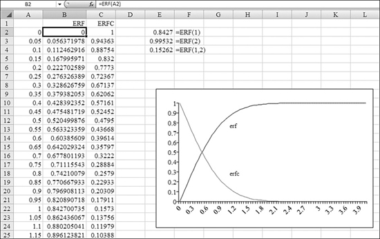
Syntax: ERF(x)

In this first syntax, the ERF function returns the error function for x.

Syntax: ERF(lower_limit,upper_limit)

In this second syntax, the ERF function returns the error function integrated between lower_limit and upper_limit. This function takes the following arguments:

• lower_limit—This is the lower bound for integrating ERF.
• upper_limit—This is the upper bound for integrating ERF. If any argument is nonnumeric, ERF returns a #VALUE! error. If any argument is negative, ERF returns a #NUM! error.

Syntax: ERFC(x)

The ERFC function returns the complementary ERF function integrated between x and infinity. The argument x is the lower bound for integrating ERF. If x is nonnumeric, ERFC returns a #VALUE! error. If x is negative, ERFC returns a #NUM! error.

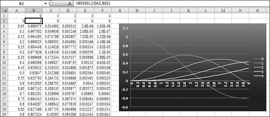
Calculating the BESSEL Functions

The BESSEL function is useful in many physics applications that involve solving classical partial differential equations in cylindrical coordinates. Excel offers four versions of the BESSEL function:

• BESSELJ—This solves the BESSEL function of the first kind. You use this function to solve BESSEL differential equations that are nonsingular at the origin.
• BESSELY—This solves the BESSEL functions of the second kind. You use this function to solve BESSEL differential equations that are singular at the origin. The BESSEL functions of the second kind are sometimes called Weber or Neumann functions.
• BESSELI—This solves the modified BESSEL differential equation. It is closely related to BESSELJ.
• BESSELK—This solves the modified BESSEL function of the second kind. This function is also known as the Basset function, Macdonald functions, or BESSEL functions of the third kind.

Each Bessel function takes two required arguments:

• x—This is the value at which to evaluate the function.
• n—This is the order of the BESSEL function. If n is not an integer, it is truncated.

If x is nonnumeric, BESSELI returns a #VALUE! error. If n is nonnumeric, BESSELI returns a #VALUE! error. If n is less than 0, BESSELI returns a #NUM! error.

Figure 27.48 shows the BESSELJ and BESSELY functions for orders of n from 0 through 4.

Figure 27.48. This chart shows the BESSELJ and BESSELY functions.

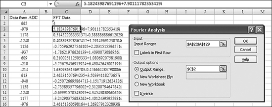
Using the Analysis Toolpack to Perform Fast Fourier Transforms (FFTs)

Many of the engineering functions have been promoted from the Analysis Toolpack to the regular version of Excel. However, one feature is left orphaned in the Analysis Toolpack. If you need to perform Fourier analysis, you should install the Analysis Toolpack.

→  See “Installing the Analysis Toolpack in Excel 2007,” page 712, in Chapter 26.

Fourier transforms are used to evaluate the output of an analog-to-digital conversion (ADC). To perform a Fourier Transform, you follow these steps:

1. Import your ADC data into Excel. The ADC record should contain a specific number of records that are powers of 2, up to 4,096 (for example, 2, 4, 8, 16, 32, 64, 128, 256, 512, 1,024, 2,048, or 4,096).
2. Make sure the Analysis Toolpack is installed.
3. From the Data ribbon, choose Data Analysis.
4. Select Fourier Analysis and click OK. The Fourier Analysis dialog appears.
5. In the Fourier Analysis dialog, select your ADC data as the input range. If your input range includes a heading, check the Labels in First Row box. In this case, your data must be (n^2) + 1 records long.
6. Choose the top-left cell of the output range.
7. Leave the Inverse check box unchecked. (It is used to convert FFT numbers in imaginary format back to the ADC format).
8. Click OK to perform the transformation.

In Figure 27.49, the original data is in Column A, and the transformed data is in Column C.

Figure 27.49. The Fourier analysis tool can convert ADC data to complex Fourier numbers.