
Chapter 28. Connecting Worksheets, Workbooks, and External Data
In this chapter
Connecting to a Worksheet in Another Workbook 800
Connecting to Data on a Web Page 805
Setting Up a Connection to a Text File 809
Setting Up a Connection to an Access Database 812
Setting Up SQL Server, XML, OLE DB, and ODBC Connections 813
In Chapters 20, “Understanding Formulas,” and 21, “Controlling Formulas,” you learned how to set up formulas that calculate based on values within one worksheet. It is also very easy to connect a worksheet to several other worksheets or to connect various workbooks. Excel 2007 offers easier-than-ever ways to connect a worksheet to data from the Web, data from text files, or data from databases such as Access.
In this chapter, you’ll learn how to do the following:
- Connect two worksheets
- Connect two workbooks
- Manage links between workbooks
- Connect to Web data
- Connect to text data
- Connect to Access data
- Manage connections
Connecting Two Worksheets
Although Excel 2007 offer 17 billion cells on every worksheet, it is fairly common to separate any model onto several different worksheets. You might choose to have one worksheet for each month in a year or to have one worksheet for each functional area of a business. For example, Figure 28.1 shows a workbook with worksheets for revenue and expenses. Because different departments might be responsible for the functional areas, it makes sense to separate them into different worksheets. Eventually, though, you will want to pull information from the various worksheets into a single summary worksheet.
Figure 28.1. Different functional areas need to work on budgets for revenue and expenses, so revenue and expenses are kept on separate worksheets.

To create a formula that pulls data from another worksheet, you enter an equals sign to begin the formula, as shown in Figure 28.2.
Figure 28.2. To link to a cell on another worksheet, you start with an equals sign.

Rather than try to remember the exact syntax, you can simply point to the correct cell. So after you type the equals sign, click the desired worksheet tab. Using the mouse, click on a cell to get the value from that cell. In Figure 28.3, Excel builds the formula =Revenue!F6 in the formula bar. Excel waits for you to either press the Enter key to accept the formula or press another operator key in order to add other cells to the formula.
Figure 28.3. Excel builds the syntax for you.

When you press the Enter key to accept the formula, Excel jumps back to the starting worksheet. The desired figure is carried through to the worksheet.
Note
The formula that Excel builds is a relative formula. You can easily copy B5 to B6 in order to retrieve the 2008 budget for revenue.
You continue this process until you have built a formula for each cell on the Summary worksheet. Note that it is okay to include an external cell as the argument for a function. Figure 28.4 shows the formula for each cell on the Summary worksheet.
Figure 28.4. A variety of formulas can link to various worksheets.

Syntax Differences When a Worksheet Name Contains Spaces
In the examples in the previous section, the syntax is as follows:
=sheetname!celladdress
This syntax changes when one of the worksheet names contains a space. In this case, you must surround the worksheet name in apostrophes, like this (see Figure 28.5):
='sheet name'!celladdress
Figure 28.5. If a worksheet name contains a space, you must surround the name with apostrophes.

Connecting to a Worksheet in Another Workbook
It is possible to set up links from a worksheet in one workbook to a worksheet in another workbook. Excel does an excellent job of managing these links and is even able to update values in the destination workbook when the source workbook is closed. It is easiest to create these links while both workbooks are open.
Say that a co-worker in another department maintains a workbook. You need to pull the sum of a few numbers from that workbook into your workbook. Your co-worker’s workbook is referred to as the source workbook and your workbook is referred to as the destination workbook. To set up a formula in the destination workbook, which pulls data from the source workbook, follow these steps:
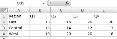
- Open the destination workbook and leave it open in the background. In Figure 28.6, the destination workbook is the RegionTotals workbook.
Figure 28.6. To pull values from this workbook into another workbook, it is easiest to have this workbook open in the background.
- Open the destination workbook. In the destination workbook, add a formula. Start by typing =SUM( in that cell (see Figure 28.7).
Figure 28.7. Rather than typing the reference at this point, it is easier to point to the cell.

- In the Windows taskbar, click the icon for the source workbook. Using the mouse, click and drag to select the target cells. In the example in the figure, Excel shows that the provisional formula is =SUM([RegionTotals.xlsm]Quota!$B$2:EE$2.
Note
When you build a link from one worksheet to another worksheet in the same workbook, Excel defaults to using a relative reference for the cell. In Figure 28.8, note that Excel defaults to entering an absolute reference when the selected reference is in another workbook. At the point shown in the figure, you can press F4 three times to return to a relative reference.
Figure 28.8. After you select the cells in another workbook, Excel defaults to an absolute reference.

- To complete the formula, type the closing parenthesis and then press Enter. You can now copy the formula to other cells in your target workbook.
Syntax Variations When Creating Links
There are some key syntax variations you must understand when creating links between worksheets and/or workbooks:
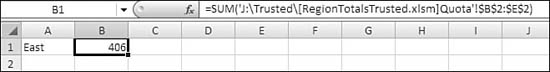
- When the worksheet name contains a space, Excel automatically adds apostrophes around the workbook name and sheet name. An example is =SUM(’[RegionTotals.xlsm]Forecast Quota’!B4:E4).
- Excel also adds apostrophes when the filename contains a space. An example is =SUM(’ [Region Totals.xlsm]ForecastQuota’!B4:E4).
- When Excel refers to a file such as [RegionTotals.xlsm], you can assume that the file is currently open. When you close the linked file, Excel updates the formula in the linking workbook to include the complete pathname. For example, =SUM(’C:[Region Totals.xlsm]Quota’!$B$2:$E$2).
- When you save the linking file, Excel notes the current location of all the linked workbooks. Excel has a problem noting the location if you’ve linked to a workbook that is not yet saved.
Creating Links to Unsaved Workbooks
Build a formula that links to a source workbook where the source workbook has not been saved. This formula might point to Book1 or Book3 or a workbook such as that. Attempt to save the destination workbook. Figure 28.9 shows a link to a new Book3 workbook. When you attempt to save the destination workbook, Excel presents a dialog that asks Is It OK to Save with References to Unsaved Documents? In general, you should cancel the save, switch to the unsaved source workbook, and then select File, Save As to save the file with a permanent name. Then you can come back to save the linking workbook.
Figure 28.9. A link to an unsaved workbook.
Using the Links Tab on the Trust Center
By default, Excel applies security settings that frustrate your attempts to pull values from closed workbooks. Consider the following scenario using two workbooks labeled Workbook A and Workbook B:
- Establish a link from Workbook A to Workbook B.
- Save and close Workbook A.
- Make changes to Workbook B. Save and close Workbook B.
- On a future day, open Workbook B.
- Open Workbook A.
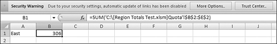
- In this case, the new values in Workbook B automatically flow through to Workbook A. However, if you attempt to later open Workbook A before opening Workbook B, you see a message below the ribbon and above the formula bar, as shown in Figure 28.10: Security Warning. Due to Your Security Settings, Automatic Update of Links Has Been Disabled. You can click either Enable Content or Trust Center.
Figure 28.10. New in Excel 2007, linked files are untrusted by default.
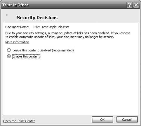
If you click Enable Content, a new Trust in Office dialog box offers you the security options to either leave the content disabled or to enable the content. It is a little unclear how updating the link to an external cell can make your document unsecure. If you want to see the current values from the closed workbook, you have no choice other than to enable this content, as shown in Figure 28.11.
Figure 28.11. You have to overlook this ominous warning from Microsoft to have Excel get a linked value from a closed workbook.
Even more annoying, choosing Enable This Content is a temporary setting. The next time you open the workbook, Excel will again disable the automatic update of links.
To permanently allow the updating of links, you need to click the Trust Center button, choose the External Content section, and then select Enable All Workbooks Links, as shown in Figure 28.12.
Figure 28.12. To permanently allow links, choose Enable All Workbook Links in this dialog.

Caution
If you choose to disable all links, Excel does not even warn you that you are seeing the wrong numbers. In Microsoft’s attempt to prevent some obscure chance of a virus, these new settings will cause enough inadvertent errors to cause a Sarbanes-Oxley auditor to sweat.
Overcoming the Trust Center by Using a Trusted Location
There is a simple way to prevent the Trust Center from getting in your way. For example, if you generally store the budget documents in a c:Budget folder on your hard drive, you can add this entire folder to your trusted locations. When the linking file is stored in a trusted location, the links automatically update, no matter what settings you have in the Links section of the Trust Center.
To add a folder to your trusted locations, you follow these steps:
- Choose File, Excel Options, Trust Center.
- Click Advanced Trust Center Settings, followed by Trusted Locations and Add New Location.
- Click the Browse button and navigate to C:Budget.
Note
Curiously, having the linking workbook in a trusted location is sufficient. Even if this workbook is linking to a file in a nontrusted location, Excel happily updates the links.
Opening Workbooks with Links to Closed Workbooks
Say that you have saved and closed the linking workbook. You update numbers in the linked workbook. You save and close the linked workbook. Later, when you open the linking workbook, Excel asks if you want to update the links to the other workbook. If you created both workbooks and you have possession of both workbooks, it is fine to allow the workbooks to update.
Dealing with Missing Linked Workbooks
If you received a linking workbook via email and do not have access to the linked workbooks, Excel alerts you that the workbook contains one or more links that cannot be updated. In this case, you should click Continue in the dialog box shown in Figure 28.13.
Figure 28.13. This message means that the linked workbook cannot be found. It shows up most often when someone mails you only the linking workbook.

You also get this message if the linked workbook was renamed, moved, or deleted. In that case, you should click the Edit Links button to display the Edit Links dialog (see Figure 28.14). Then you should click the Change Source button to tell Excel that the linked workbook has a new name or location. Finally, you need to click the Break Link button to change all linked formulas to their current values.
Figure 28.14. You can manage or change links by using this dialog.

Preventing the Update Links Dialog from Appearing
Say that you need to send a linking workbook to a co-worker. You want your co-worker to see the current values of the linking formulas without having the linked workbook. In this case, you want the co-worker to click Continue in Figure 28.13. However, some newer Excel customers think that every warning box is a disaster, so you might prefer to suppress that box for your co-worker. To do so, you follow these steps:
- On the Data tab, in the Manage Connections group, choose Edit Links to Files.
- In the lower-left corner of the dialog that appears, click the Startup Prompt button. The Startup Prompt dialog appears.
- Select Don’t Display the Alert and Don’t Update Automatic Links (see Figure 28.15).
Figure 28.15. You can prevent others from seeing the Update Links message.

Of course, after emailing the workbook to your co-worker, you need to redisplay the Startup Prompt dialog and change it back so that you will get the updated links.
Connecting to Data on a Web Page
Many Web pages comprise many tables of data. Any time you see columns of numbers or columns of data, it is very likely that you are seeing the results of a table. Usually the only things not in a table are paragraphs of body copy. And usually, there would be no need to update this information on a daily basis. Excel 2007 makes it even easier than past versions of Excel to link your Excel worksheet to a table on any Web page.
Setting Up a Connection to a Web Page
To set up a connection between a worksheet and a Web page, you follow these steps:
- Find a section of the worksheet that has several blank rows and blank columns. (Depending on the size of the selected sections of the Web page, you could return many rows or columns of data.)
- On the Data ribbon, choose From Web from the Get External Data group. Excel opens the New Web Query dialog. This dialog looks remarkably like a mini Web browser, and it even opens to your default home page from Internet Explorer. However, as shown in Figure 28.16, the rendered Web page includes several yellow boxes with black arrows. These arrows indicate the tops of various tables on the page.
Figure 28.16. Notice the arrows indicating available tables on the Web page.

- Using the search bar or the address bar, navigate to the selected Web page. For example, to retrieve stock quotes, you might use http://finance.yahoo.com.
- If the Web page has a form, enter any values needed by the form. In this example, you would enter your desired ticker symbols into the Yahoo Get Quotes box and then press Go. The resulting Web page will probably have many tables. The Yahoo quotes page has at least 14 tables, many of which are tables that display advertisements.
- Hover the mouse over various yellow and black arrows. Excel highlights the entire range of each table, as shown in Figure 28.17.
Figure 28.17. You select the table that contains the data for the worksheet.

- When you find the table that contains the information that you want, click that arrow. The arrow changes to a green checkmark, as shown in Figure 28.17.
- In the upper-right corner of the New Web Query dialog, click the Options button. The Web Query Options dialog appears (see Figure 28.18).
Figure 28.18. Most of the time, you want unformatted text.
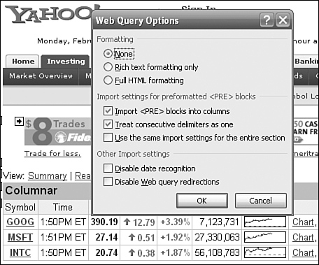
- Select whether the data from the Web page should be retrieved as text only or whether to have full HTML formatting in the results. Then click OK.
- Click the Import button in the lower-right corner of the New Web Query dialog. Excel displays the Import Data dialog, which allows you to confirm the output location for the data from the Web query. If desired, click the Properties button to set up automatic refreshing of the Web data. The Connection Properties dialog appears (see Figure 28.19).
Figure 28.19. You control the refresh rate for the Web query on this dialog.
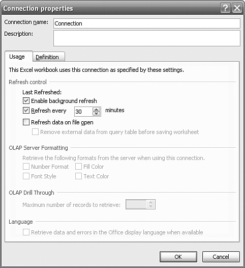
- Use the Connection Properties dialog to set refresh options. For example, you can have the Web query refreshed every so many minutes, and you can also have the Web data refreshed when a file opens. This way, you can retrieve new data each day when you open the file. When you are done selecting options on this dialog, click OK. You will briefly see a bit of Web query code appear in the worksheet at your destination location. If your Internet connection is working, this is soon replaced by the data from the Web page, as shown in Figure 28.20.
Figure 28.20. The results of the Web query are imported to your workbook.

Note in Figure 28.20 that all the Get External Data options in the ribbon are disabled. This happens when your cell pointer is located in external data. To set up a new Web query on the same worksheet, you simply move the cell pointer to a cell outside the retrieved data; for example, Cell A9 would be safe in the worksheet shown in Figure 28.20.
Managing Cell Properties for Web Queries
After you have retrieved a Web query, you can select a single cell in the query and choose Properties from the Manage Connections group on the Data ribbon. The External Data Range Properties dialog appears. As shown in Figure 28.21, this legacy dialog box includes additional properties for the query. In the Data Formatting and Layout section, you can choose options to preserve cell formatting and adjust column widths. Most importantly, you can specify that if the query returns more rows tomorrow, any formulas adjacent to the Web query should be expanded.
Figure 28.21. This dialog box includes formatting and formula properties.

Setting Up a Connection to a Text File
It is possible to load data from a text file into Excel using the connection group. Follow these steps:
- On the Data ribbon, choose the From Text icon in the Get External Data group. The Import Text File dialog appears.
- Browse to and select your text file. Excel launches the familiar Text Import Wizard – Step 1 of 3, where you can specify that the text is either delimited or fixed width. (Delimited text is text in which each column is separated by a character such as a comma or a tab. Fixed-width data is where each field is neatly lined up when viewed in a monospace font such as Courier New.)
- Choose Delimited, as shown in Figure 28.22, and then click Next.
Figure 28.22. You navigate through the Text Import Wizard to set up a connection to a text file.

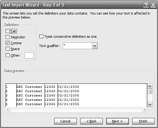
- In step 2 of the wizard, change the Excel default Tab character between fields to a comma, as shown in Figure 28.23. (You may occasionally encounter files with a delimiter such as a pipe (|) or some other character. You can specify such a delimiter by choosing the Other check box and then specifying the character.)
Figure 28.23. You specify the delimiter character in step 2.
- In step 3, specify the field type for each field and whether certain fields should be skipped.
- If you have a column of numbers where a leading zero needs to be preserved (for example, the zip code of Fort Kent, Maine, needs to stay as 04743 instead of being converted to 4743), choose Text as the field type for the zip code field.
- Click the Advanced button to specify the characters used for thousands and decimal separators (see Figure 28.24). You can also specify that the minus appears after the number.
Figure 28.24. You select field types in step 3.

- Click Finish. The Import Data dialog appears.
- Specify a starting cell for the data, as shown in Figure 28.25.
Figure 28.25. In addition to specifying a starting cell, click the Properties button.

- Click the Properties button. The Properties dialog appears.
- Determine whether to have Excel ask you for the filename each day or if you should use the same file name each day. If your IT department is putting out an inventory.txt file every day, you will always want to connect to inventory.txt. Instead, your IT department might be exporting inv070217.txt today and inv070218.txt tomorrow. In that case, you would want Excel to ask you for a filename during every refresh. As shown in Figure 28.26, Excel defaults to Prompt for File Name on Refresh. If your filename will be the same and in the same folder every day, uncheck this default setting.
Figure 28.26. By default, Excel asks you for the filename during every refresh from a text connection. Turn this off if your file will be in a consistent location with the same name.

- Accept the location for the import. Excel brings in all the records from the text file.
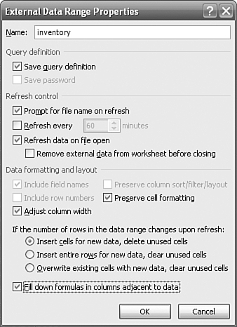
- Click the Properties icon under Manage Connections on the Data tab in order to access additional properties for the query. In particular, you can control how Excel will handle new records each day and ask that any formulas in adjacent cells be extended as needed. The options for column sort/filter/layout are disabled for a text file. Figure 28.27 shows the External Data Range Properties dialog.
Figure 28.27. You can choose refresh options for the text connection.
Setting Up a Connection to an Access Database
Although Excel can now handle 1.1 million rows, you might encounter larger datasets that need to be stored in Access. You can connect to these larger datasets. You can create a connection to any table in an Access database. Here’s what you do:
- On the Data ribbon, in the Get External Data group, choose From Access.
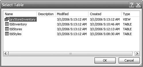
- Browse to select the .mdb file to which you want to link. You are then given an opportunity to choose any one table or query from the database. Each query is listed in the Type column as VIEW, as shown in Figure 28.28.
Figure 28.28. Using an Access connection, you can import a table or a predefined query.
- Choose whether your data should be imported as a table or used in a pivot table. With the Access connection, there is an additional option as shown in Figure 28.29. You can have the table imported to a regular table, or you can ask for the data to be used as the data source for a pivot table report. When the Access data is delivered to Excel, it is automatically set up as an Excel table with default formatting, as shown in Figure 28.30.
Figure 28.29. Access connections can be returned as a table or used as the source in a pivot table report.

Figure 28.30. By default, Excel treats the data with Excel 2007’s table formatting and features.

Note
Note that if you select a query in Access, there might be a delay as the query is calculated. Excel displays a Getting Data... message in the table while the calculation is in process.
→ To learn more about pivot tables, see Chapter 11, “Formatting Pivot Table,” page 215.
Setting Up SQL Server, XML, OLE DB, and ODBC Connections
Although Excel 2007 offers icons for Access, Web, and text connections, you can actually connect to a wide variety of other data sources. You access all these sources by clicking the From Other Sources icon on the Data ribbon. When you choose this option, you are presented with five choices, as shown in Figure 28.31.
Figure 28.31. Excel can connect to SQL Server, Analysis Services, XML, OLE DB data sources, or ODBC through Microsoft Query.

SQL Server is Microsoft’s structured query language database. Typically, when applications get too big to run smoothly in Microsoft Access, they will be migrated to the more robust SQL Server platform. Because SQL Server is a Microsoft product, connecting to SQL Server is easy. To connect, you will need the Server name, a userid, and a password.
Analysis Services is Microsoft’s cube functionality, currently marketed as SQL Server Analysis Services. A cube database represents data along three or more dimensions. To connect, you will need the Server name, a userid, and a password.
XML stands for Extensible Markup Language. This is a simple text file that includes both data and tags used to identify the data. An example illustrating a connection to XML data is shown in the next section.
OLE-DB stands for Object Linking and Embedding for Databases. This is a Microsoft interface written in the COM environment that allows Windows-based applications to access a wide variety of database types. Consult your database administer for required settings to connect through OLE-DB. Microsoft Query is an older technology that uses Open Database Connectivity (ODBC). If your company has implemented a non-Microsoft platform, ODBC is the interface that allows other programs such as Excel to connect to the database. Typically, the administrator of the system will be able to provide you with a connect string that you will use to access the other system’s data. Microsoft Query also provides a method for Excel to build SQL queries against Access databases. For an example, see “Connecting Using Microsoft Query” later in the chapter.
Connecting to XML Data
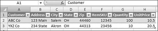
In the future, you will find more and more datasets based on XML. In reality, XML is like a CSV (comma-separated value) file on steroids. You can create or edit XML files by using Notepad. The difference between a CSV file and an XML file is that each field in XML contains a field identifier. This allows you to intelligently import only certain fields into a spreadsheet. Figure 28.32 shows a simple XML file that has two records.
Figure 28.32. In this XML file seen in Notepad, note that each field starts and ends with <fieldname> and </fieldname> tags.

In addition to the actual XML file, it is possible to have a definition document known as an XSD file or a database schema. You may also have one or more XSL files that are used to transform the data. But as long as you have at least one XML file, Excel will be happy to infer a schema, as shown in Figure 28.33.
Figure 28.33. Without a schema file, Excel is limited to importing the data as a table. Luckily, Excel creates a schema file for you.

As you can see in Figure 28.34, the data is then imported as an Excel table. This is pretty basic functionality. By using a trick in the VBA Editor, however, you can actually retrieve the schema and save it to allow Excel to do more XML tricks.
Figure 28.34. The data from Figure 28.32 after being imported to Excel.
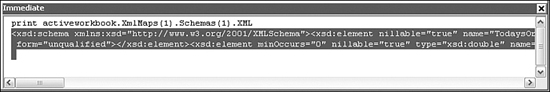
After Excel has imported the data, you can retrieve the schema by using the VBA Editor. To do so, you follow these steps:
- Press Alt+F11 or click the VBA Editor icon on the Developer ribbon. The VBA Editor appears.
- In the VBA Editor, press Ctrl+G to display the Immediate pane.
- In the Immediate pane, type this line:
print activeworkbook.XmlMaps(1).Schemas(1).XML
Then press Enter. Excel responds by printing the entire schema for the XML file, as shown in Figure 28.35.
Figure 28.35. Excel will reply with the Schema.
- Copy this text into a blank Notepad file and save as test.xsd in the same directory as the XML file.
Figure 28.36 shows the complete schema in Notepad, with WordWrap turned on.
Figure 28.36. You save the schema to enable additional XML features in Excel.

Connecting Using Microsoft Query
The From Access icon on the Data ribbon allows you to retrieve all fields from any Access table or predefined query. There may be times when you want to join Access tables, filter records, or select only a subset of fields from a query. Excel 2007 offers the old Microsoft Query product for building such connections.
To build a new query against a table in an Access database, follow these steps:
- In Excel 2007, choose Data, Get External Data, From Other Sources, From Microsoft Query. The Choose Data Source dialog appears.
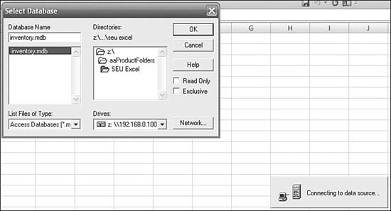
- Select MS Access Database, as shown in Figure 28.37. Click OK. The Select Database dialog will appear. (Note: The Choose Data Source dialog differentiates between Access and Access 2007 databases. If your data is in an Access 2007 database, choose MS Access 12.0 Databases instead.)
Figure 28.37. Choose MS Access Database in the Choose Data Source dialog.

- In the Select Database dialog, choose the Access database, as shown in Figure 28.38. (Although Office 2007 was supposed to be a complete rewrite, it is apparent that no one has updated this Windows 3.1–style dialog box in many years.) The Query Wizard dialog appears.
Figure 28.38. You select the Access database.
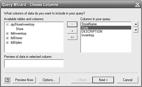
- Choose to include particular fields from any table or query in the database. You Choose fields on the left side of the dialog and click the > button to move them to the right side of the dialog, as shown in Figure 28.39.
Figure 28.39. You select fields to be included in the query.
- In the next step of the Query Wizard, set up filters for the query. In Figure 28.40, the filter is defined as only items where the inventory is greater than five.
Figure 28.40. You define filters for the query.

- In the next step of the Query Wizard, specify up to three sort fields for the query, as shown in Figure 28.41.
Figure 28.41. You specify sort criteria.

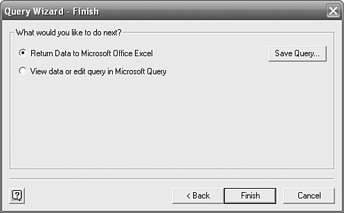
- In the final step of the Query Wizard, specify that you want to return the data to Microsoft Office Excel, as shown in Figure 28.42. You will are presented with an Import dialog that is similar to the one shown earlier.
Figure 28.42. You return the data to Excel.
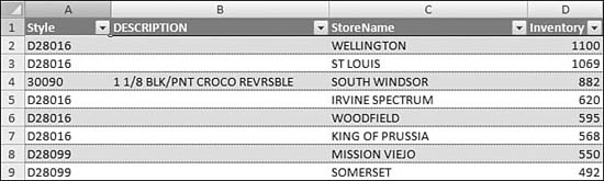
Contrast the current example with the previous example in “Setting Up a Connection to an Access Database.” Although the previous example and this example use the same query from Access, the Microsoft Query option enables you to retrieve only the records with more than five items in inventory. The overhead involved in returning few records causes the query to run significantly faster. As shown in Figure 28.43, the data is returned in a sorted manner.
Figure 28.43. The final results from the MS Query connection.
Managing Connections
The Data ribbon includes a group called Manage Connections. As shown in Figure 28.44, this group includes an option to refresh all connections. Although the icon says Refresh All, there is a drop-down available where you can choose to refresh only the current query or to view properties for a connection.
Figure 28.44. You have one-click access to refreshing all connections.

Clicking the Connections icon brings up a summary of all the Web, text, Access, or ODBC connections in your workbook. This is a fantastic improvement in Excel 2007. As shown in Figure 28.45, you can click any connection in the top and then follow the hyperlink Click Here to See Where the Selected Connections Are Used in order to jump to the worksheet range that houses the results of the connection.
Figure 28.45. The new Workbook Connections dialog provides one stop to see all connections in the workbook.

While this new dialog is very nearly a one-stop source for all external links, you might be disappointed to learn that links to other workbooks are not included in this dialog. You have to select Edit Links to Files from the Manage Connections group in order to display the Edit Links dialog, where you can check the status of any workbook links as well as maintain the link location, break the links, or adjust the startup prompt.
Excel offers fantastic connections. Although users have been able to link to Access databases for several versions, Excel 2007’s improved support for SQL Server, XML, ODBC, text, Web, and Access data is unparalleled. The following Excel in Practice sidebar talks about setting up a connection to one of the newest data stores: an Excel 2007 workbook with half a million records.
Figure 28.46. Use Edit Links to manage formula links between workbooks.

Excel in Practice: Defining a Connection to a Separate Closed Workbook
While you can write formulas that link to external closed workbooks, those formulas cannot reference more than 10,000 cells. This is a serious limitation now that you can have more than a million rows in the external worksheet.
Rather than using simple linking via a formula, you can treat the other Excel file as a database file and connect to it using the Connection Manager! This technique will allow you to run queries against millions of cells in the external workbook.
For example, Figure 28.47 shows an Excel worksheet with more than 748,000 records. Link formulas would not be able to access more than 2% of the rows in this workbook. Using a connection will overcome this limitation.
Figure 28.47. With 20 columns, this worksheet contains 15 million cells.

To create a connection to the external workbook, follow these steps.:
- From a blank workbook, choose Data, Get External Data, From Other Sources, From Microsoft Query. In the Choose Data Source dialog that appears, choose Excel 2007 Connection (also known as MS Excel 12.0 Files).
- In the Select Workbook dialog, choose the Excel file and click OK.
- In the next three Query Wizard dialogs, select your fields, the filter, and the sort.
- In the final step, choose the option to view the query in Microsoft Query. The Microsoft Query dialog appears.
- In the Microsoft Query dialog, choose View, Query Properties. The Query Properties dialog appears (see Figure 28.48)
Figure 28.48. Grouping records will return one record per Region and Product.

- Choose the Group Records check box and click OK. This will tell the query to return a summary dataset, totaling numeric fields for each unique combination of key fields. You will specify which fields to group and sum in the next two steps.
- Select the Sum of Quantity heading in the lower half of the screen. Click the Sigma button in the toolbar to toggle through Sum, Min, Max, and Normal. Choose Sum as shown in Figure 28.49.
Figure 28.49. You select a sum property for each column.

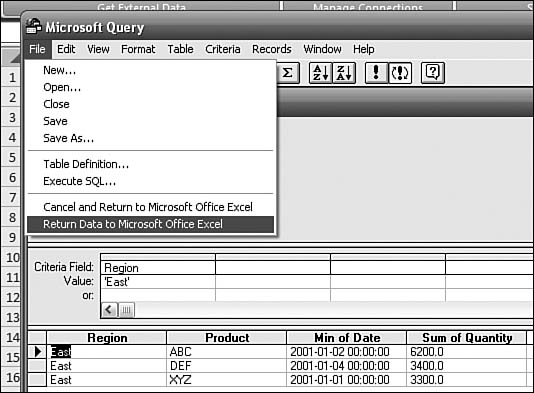
- Choose File, Return Data to Microsoft Excel, as shown in Figure 28.50.
Figure 28.50. You close Microsoft Query and return the data.
You now have a refreshable data connection to an external Excel workbook that has 750,000 records.
Figure 28.51. This is a three-line summary from the 750,000-record external workbook.
