Chapter 21. Controlling Formulas

In this chapter

Formula Operators 410

Understanding Error Messages in Formulas 414

Using Formulas to Join Text 415

Copying Versus Cutting a Formula 418

Automatically Formatting Formula Cells 419

Using Date Math 421

Troubleshooting Formulas 423

While you can go a long way with simple formulas, it is also possible to build extremely powerful formulas. The topics in this chapter will explain the finer points of formula operators, date math, and how Excel distinguishes between cutting and copying cells referenced in formulas.

Formula Operators

Excel offers the mathematical operators shown in Table 21.1.

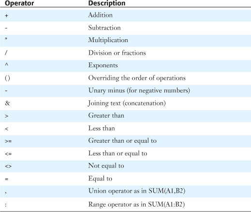
Table 21.1. Mathematical Operators

The Order of Operations

When a formula contains many calculations, Excel will evaluate the formula in a certain order. Rather than calculating from left to right as a calculator might, Excel will perform certain types of calculations such as multiplication before calculations such as addition.

You can override the default order of operations with parentheses. If you don’t use parentheses, Excel uses the following order of operations:

1. Unary minus is evaluated first.
2. Exponents are evaluated next.
3. Multiplication and division are handled next, in a left-to-right manner.
4. Addition and subtraction are handled next, in a left-to-right manner.

The following sections provide some examples of order of operations.

Unary Minus Example

The unary minus is always evaluated first. Think about when you use exponents to raise a number to a power. If you raise -2 to the second power, Excel calculates -2 × -2, which is +4. So the formula =-2^2 evaluates to 4.

If you raise -2 to the third power, Excel calculates (-2) × (-2) × (-2). Multiplying -2 by -2 results in +4, and multiplying +4 four by -2 results in -8. So the simple formula =-2^3 generates -8.

You need to understand a subtle but important distinction. When Excel encounters the formula =-2^3, it evaluates the unary minus first. If you want the exponent to happen first and then have the unary minus applied, you have to write the formula as =-(2^3). However, in a formula such as =100-2^3, the minus sign is considered to be a subtraction operator and not a unary minus sign. In this case, 2^3 is evaluated as 8, and then 8 is subtracted from 100.

Figure 21.1 shows the results of three formulas involving raising -2 to various powers.

Figure 21.1. Beware the unary minus. Three very similar formulas have different results, depending on where the minus sign occurs.

Addition and Multiplication Example

The order of operations is important when you are mixing addition/subtraction with multiplication/division. For example, if you want to add 20 to 30 and then multiply by 1.06 to calculate a total with tax, the following formula leads to the wrong result:

=20+30*1.06

The result you are looking for is 53. However, the Evaluate Formula dialog shows that Excel calculates the formula =20+30*1.06 like so (see Figure 21.2):

1.06 × 30 = 31.8

31.8 + 20 = 51.8

Figure 21.2. The underline indicates that Excel does the multiplication first.

Excel’s answer is $1.20 less than expected because the formula is not written with the default order of operations in mind.

To force Excel to do the addition first, you enclose the addition in parentheses:

=(20+30)*1.06

Figure 21.3 shows the second step in the Evaluate Formula dialog for this formula. The addition in parentheses is done first, and then 50 is multiplied by 1.06 to get the correct answer of $53.

Figure 21.3. Excel evaluates the operation in parentheses first.

Stacking Multiple Parentheses

If you need to use multiple sets of parentheses when doing math by hand, you might write math formulas with square brackets and curly braces, like this:

{3-[6*4*3-(3-6)+2]/27}*14

In Excel, you simply use multiple sets of parentheses, as follows:

=(3-(6*4*3-(3-6)+2)/27)*14

Formulas with multiple parentheses in Excel are therefore very confusing. Excel does two things to try to improve this situation:

• First, as you are typing a formula, Excel colors the parentheses in a set order: black, dark green, purple, brown, light green, orange, magenta, blue, medium green, purple, brown, light green, and so on. If you bump the zoom up on your screen to 400%, you might actually be able to make out the color differences in the parentheses. However, at the normal zoom, the colors black, green, purple, and brown are all dark, and it is difficult to tell one from the other.
• When you type a closing parenthesis, Excel shows the opening parenthesis in bold for a fraction of a second. This would be more helpful if Excel kept the opening parenthesis in bold for 5 seconds or 20 seconds. But at about half a second, it is nothing more than a frustrating reminder that your reflexes are not fast enough. Figure 21.4 attempts to show the bolded condition at a ridiculously high zoom.

Figure 21.4. This screen shot shows that after you type the fifth closing parenthesis, the eighth opening parenthesis is briefly shown in bold.

Understanding Error Messages in Formulas

Don’t be frustrated when a formula returns an error result. These eventually happen to everyone. The key is to understand the difference between the various error values so that you can begin to troubleshoot the problem.

As you enter formulas, you might encounter a number of errors, including these:

• #VALUE!—This error indicates that you are trying to do math with nonnumeric data. For example, the formula =4+apple will return a #VALUE! error. This error also occurs if you try to enter an array formula and fail to use Ctrl+Shift+Enter, as described in Chapter 29, “Using Super Formulas in Excel.”
• #DIV/0!—This error occurs when a number is divided by zero—that is, when a fraction’s denominator evaluates to zero.
• #REF!—This error occurs when a cell reference is not valid. It can occur when one of the cells referenced in the formula has been deleted. It can also occur if you cut and paste another cell over a cell referenced in this formula. If you are using Dynamic Data Exchange (DDE) formulas to link to external systems and those systems are not running, you may also get this error.
• #N/A!—This error occurs when a value is not available to a function or a formula. #N/A! errors most often occur as a result of key values not being found during lookup functions. They can occur as a result of HLOOKUP, LOOKUP, MATCH, or VLOOKUP. They can also result when an array formula has one argument that is not the same shape as the other arguments or when a function omits one or more required arguments. Interestingly, when an #N/A! error enters a range, all subsequent calculations that refer to the range have a value of #N/A!.
• ######—This is not really an error. It simply means that the result is too wide to display in the current column width, so you need to make the column wider to see the actual result.

In Figure 21.6, cell E17 is a simple SUM function. It is returning an #N/A! error because Cell E11 contains the same error. Cell E11 contains the formula =D11*C11. The root cause of the problem is the VLOOKUP function in Cell D11. Because Dill cannot be found in the product table in G7:H9, the VLOOKUP function returns #N/A!.

Figure 21.6. The error in E17 is actually caused by an error two calculations earlier.

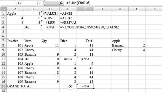
Figure 21.6 shows only a small table, so it is relatively easy to find the earlier #N/A! errors. If you were totaling 100,000 rows, however, it could be difficult to find the one offending cell. To track errors down, you follow these steps:

1. Select the cell that shows the final error. To the left of that cell, you should see an exclamation point in a yellow diamond.
2. Hover the cursor over the yellow diamond to reveal a drop-down arrow.
3. From the drop-down menu, choose Trace Error. Excel draws in red arrows pointing back to the source of the error, as shown in Figure 21.7. From the original #N/A! error in Cell D11, for example, blue arrows demonstrate what cells were causing the error.

   Figure 21.7. Choosing Trace Error reveals the cells leading to the error.

   

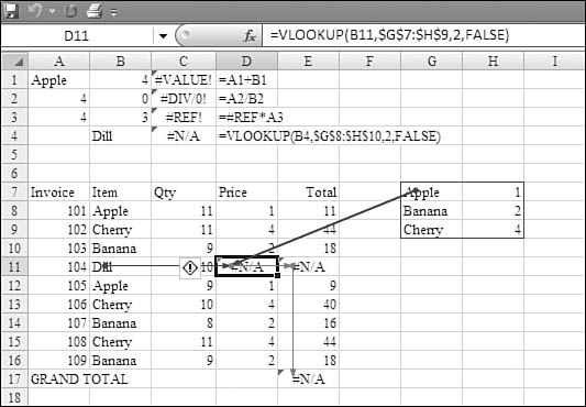
4. Repeat steps 1-3 for the cell causing the error in order to trace the original root cause of the problem.

Using Formulas to Join Text

You use the ampersand (&) operator when you need to join text. Officially, it is known as the concatenation operator.

For example, the formula =A2&B2 joins the text values shown in the two cells A2 and B2, as shown in Figure 21.8.

Figure 21.8. The & operator is used to join two text cells.

When using the & operator, you might want to include a space between the two items that are combined to improve the appearance of the output. For example, if the cells contain first name and last name, you might want to have a space between the names. To include a space between cells, you follow the & with a space enclosed in quotes (that is, &” “). As shown in Figure 21.9, the formula =A2&” “&B2 generates a better-looking result than =A2&B2. (Instead of using a space, you can also use any other text between the cells, by enclosing that text in quotes.)

Figure 21.9. You can join cells with any text in quotation marks.

Joining Text and a Number

In many cases, you can use the & operator to join text with a number. In Figure 21.10, the formula in Cell C2 joins the words “The Answer is” with the result of the calculation in Cell B2. Because Cell B2 contains an integer with no special formatting, the answer appears correctly.

Figure 21.10. Joining text with a number works if the number is formatted with general formatting.

In Figure 21.11, Cell B2 is formatted to display a currency symbol and two decimal places. When you join this value to text in Cell C2, Excel ignores the formatting in Cell B2 and shows the result with all the decimal places. A similar problem exists when you want to join text with a date. Excel ignores the fact that the text in Cell B4 is formatted as a date and shows the underlying value in Cell C4.

Figure 21.11. Joining text with a date or with formatted numbers rarely works well.

In this case, you need to discover the numeric formatting code associated with the original cell. To do so, you follow these steps:

1. Select Cell B2.
2. Press Ctrl+1 to display the Format Cells dialog.
3. On the Number tab, choose the Custom category. This reveals the actual formatting codes for the cell.

As shown in Figure 21.12, the actual formatting code for B2 is $#,##0.00. If you repeat these steps for Cell B4, you learn that the actual formatting code is m/d/yyyy.

Figure 21.12. If you choose the Custom category, you learn the actual codes used to produce the numeric format.

→  For a complete discussion of numeric formatting codes, see Chapter 32, “Formatting Worksheets,” page 891.

When you know the numeric formatting codes, you can achieve the desired effect by using those codes, enclosed in quotation marks, as the second argument of the TEXT function. In Figure 21.13, the formula in Cell C2 is =“The Answer is”&Text(B2, “$#,##0.00”). You can use a knowledge of custom numeric formatting codes to actually change the look of the joined value. In Cell C4, the new formula is =“His birthday is”&TEXT(B4, “dddd mmmm d, yyyy”).

Figure 21.13. You can use the TEXT function to replicate formatting, as in Cell C2, or to change the formatting, as in Cell C4.

Copying Versus Cutting a Formula

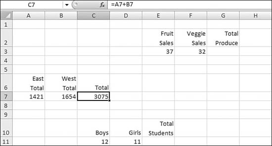
In Figure 21.14, the formula in Cell C7 references A7+B7. Because there are no dollar signs within the formula, those are relative references.

Figure 21.14. The formula in Cell C7 adds the two numbers to the left of the formula.

→  To learn more about relative versus absolute references, see “Overriding Relative Behavior: Absolute Cell References,” page 389, in Chapter 20

If you copy Cell C7 and paste it to Cell G3, the formula works perfectly, as shown in Figure 21.15.

Figure 21.15. When Cell C7 is copied to Cell G3, the formula still adds the two numbers to the left of the formula.

However, if you cut Cell C7 and paste it to a new location, the formula continues to point to Cells A7+B7, as shown in Figure 21.16. While cutting and copying are relatively similar in applications such as Word, they are very different in Excel. It is important to understand the effect of cutting a formula in Excel as opposed to copying the formula.

Figure 21.16. Using cut and paste on a formula forces the formula to continue to point to the original cells.

When you cut a formula, the formula continues to point to the original precedents, no matter where you paste it.

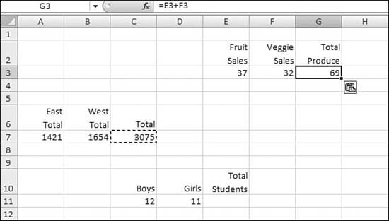
A similar rule applies to the references mentioned in a formula. The formula in Cell C7 points to A7 and B7. As long as you copy Cell A7 and/or Cell B7, you can paste them anywhere without changing the formula in C7. Figure 21.17 shows the result of copying A7:B7 for 20 rows: Nothing changes in the formula.

Figure 21.17. Copying the precedent cells from Cell C7 does not have any effect on Cell C7.

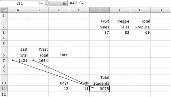
However, if you cut and paste A7:B7 to a new location, such as E5:F5, the formula in Cell C7 changes. After the paste, the formula points to the new location of the pasted cells, as shown in Figure 21.18

Figure 21.18. Cutting the precedent cells from Cell C7 causes the formula in C7 to change to reflect the new location.

Automatically Formatting Formula Cells

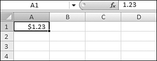
The rules for formatting the result of a formula seem to be inconsistent. Say that you have $1.23 in Cell A1, as shown in Figure 21.19.

Figure 21.19. In this case, all cells are in general format, except Cell A1.

If you enter =A1+3 in an another cell with general format, the result automatically inherits the currency format of Cell A1, as shown in Figure 21.20.

Figure 21.20. No formatting is applied to B3. Excel copies the format from Cell A1 automatically.

Note that the formatting is copied whether you use =A1+3 or =3+A1.

While Excel formulas should start with an equals sign, many desktop computer owners will start their formulas with the plus sign on the numeric keypad. This trick works to provide compatibility for people formerly using Lotus 1-2-3. If you regularly use the plus sign to start a formula, the rules for automatically formatting a cell are different. In Figure 21.21, Cell A1 has a currency format, and Cell A3 has a number format with zero decimal places. The formula in Cell C3 is +A1+A3. This result mysteriously loses the currency symbol but is formatted as a number with two decimal places. In Cell C5, the formula is reversed: +A3+A1. Here, the formula picks up the format of the last cell mentioned—the currency from Cell A1.

Figure 21.21. When starting formulas with a plus sign, the automatic formatting of cells C3 and C5 is different, depending on which cell was mentioned last.

If you enter your formulas starting with a plus sign, you can control the format by referencing a cell with similar formatting second. If you enter your formulas with an equals sign, it is best to reference the cell with similar formatting first.

Figure 21.22 compares the automatic formatting derived from entering the formula in various ways. Cell A1 is formatted as currency, A3 as number, A5 as percentage. The formulas in Column D of the left window were entered using equal signs. The formulas in Column D of the right window were entered using plus signs. In each group, a different cell was mentioned first and last in the formula. Excel automatically assigned all the formats in Column C. The formula for each Column C cell is shown to the right, in Column D.

Figure 21.22. The automatic formatting of cells C3 and C5 is different, depending on if you use = or + to start a formula.

Using Date Math

Dates in Excel are stored as the number of days since January 1, 1900. For example, Excel store the date Feb-17-2007 as 39130. In Figure 21.23, Cell A1 contains the date. Cell A2 contains the formula =A1 and has been formatted to show a number.

Figure 21.23. Although Cell A1 is formatted as a date, it really contains the number of days since January 1, 1900.

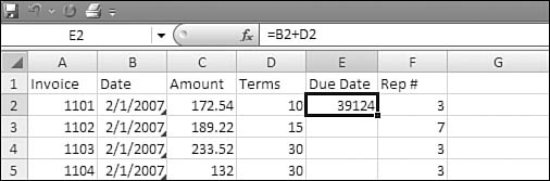
This convenient system allows you to do some pretty simple math. For example, Figure 21.24 shows a range of invoice dates in Column B. The terms for the invoice are in Column D. You can calculate the due date by adding Cells B2 and D2. Here is what actually happens in Excel’s calculation engine:

1. The date in Cell B2—2/1/2007—is stored as 39114.
2. Excel adds 10 to that number to get the answer 39124.
3. Excel formats this number as a date, to yield 2/11/2007.

Figure 21.24. When the answer is formatted correctly, Excel’s date math is very cool.

However, a frustrating problem can occur if the cell containing the formula has the wrong numeric format. For example, in Figure 21.25, you can see that Column E inherited the numeric formatting of Column D after a blank Column E was inserted. Cell E2 has exactly the same formula as Figure 21.24, but the answer here is incorrect. It’s important to recognize that dates in 2006–2009 fall in the range of 38,718 to 40,178. So if you are expecting a date answer as the result of a formula and get a number in this range, the answer probably needs to have a date format applied.

Figure 21.25. Here, the same formula as before appears to give the wrong answer. However, it is a formatting problem.

To apply a date format, on the Home Ribbon, you use the Number drop-down to choose the Date format. The answer in Cell E2 now appears correctly, as shown in Figure 21.26.

Figure 21.26. After you apply the Date format, the answer is displayed correctly.

Why doesn’t Excel automatically format all results as dates? It’s because in many cases you want to calculate the number of days between two dates. In Figure 21.27, for example, the formula in Cell C4 should correctly calculate the number of days from today until the next milestone. Although the result should be 14 days, the result in the spreadsheet is shown as the date 1/14/1900.

Figure 21.27. Here, you want the answer to be formatted as a number instead of a date.

You need to apply a numeric format to the range containing the formula. When you choose Number from the Number drop-down on the Home Ribbon, the formula appears with the correct result (see Figure 21.28).

Figure 21.28. When you apply a numeric format, the answers are correct.

Any time you are doing math between two dates, you should plan on needing to change the format of the result to be either Number or Date, depending on the situation.

→  To learn about many other useful date functions in Excel, see “Examples of Date and Time Functions,” page 490 in Chapter 23.

Troubleshooting Formulas

It is difficult to figure out worksheets set up by other people. When you receive a worksheet from a co-worker, use the information in the following sections to find and examine the formulas.

Highlighting All Formula Cells

The first technique when examing a new worksheet is to find all of the cells that contain formulas. The following steps will identify all of the formula cells in the worksheet:

1. Press F5 to display the Go To dialog.
2. In the lower-left corner of the Go To dialog, click the Special button to display the Go To Special dialog.
3. In the Go To Special dialog, choose the Formulas option button, as shown in Figure 21.29.

   Figure 21.29. The Go To Special dialog has many incredibly powerful features.

   

4. Click OK to select all formula cells.
5. To quickly highlight all the cells that contain formulas, use the paint bucket icon in the Home Ribbon to mark all the formula cells as shown in Figure 21.30.

Figure 21.30. Immediately after selecting all formulas, you choose the paint bucket icon to color the formula cells.

Seeing All Formulas

For a long time, Excel has given users the ability to see all the formulas in a worksheet. The mode that provides this functionality is called Show Formulas mode.

On most U.S. keyboards, the key just below the Esc key in the upper-left corner of the keyboard contains a tilde (~) and also a backtick (`). In previous versions of Excel, you had to press Ctrl+~ or Ctrl+` in order to toggle into and out of Show Formulas mode, in which each column is a little wider. Instead of showing the results of the formula, in Show Formulas mode, each cell shows the formula itself (see Figure 21.31). You had to press this keystroke again to return to Regular mode.

Figure 21.31. Show Formulas mode shows the formulas in the cells instead of the results. This is handy for quick formula auditing.

In addition to recognizing Ctrl+`, Excel 2007 has added an icon in the Formula Auditing section of the Formulas ribbon that enables you to toggle into and out of Show Formulas mode.

Editing a Single Formula to Show Direct Precedents

It is helpful to identify cells that are used to calculate a formula. These cells are called the precedents of the cell.

A cell can have several levels of precedents. In a formula such as =D5+D7, there are two direct precedents: D5 and D7. However, all of the direct precedents of D5 & D7 are second-level precedents of the original formula.

If you are interested in visually examing the direct precedents of a cell, follow these steps:

1. Select a cell that has a formula.
2. Press F2 to put the cell in Edit mode. In this mode, each reference of the formula is displayed in a different color. For example, the formula in Cell H5 refers to three cells. The characters F5 in the formula appear in blue and correspond to the blue box around Cell F5 in Figure 21.32.

   Figure 21.32. Editing a single formula lights up the direct precedent cells.

   

3. Visually check the formula to ensure that it is correct.

Using Formula Auditing Arrows

If you have a complicated formula, you might wish to identify direct precedents and then possibly second- or third-level precedents. You can have Excel draw arrows from the current cells to all cells that make up the precedents for the current cell. Here’s what you do:

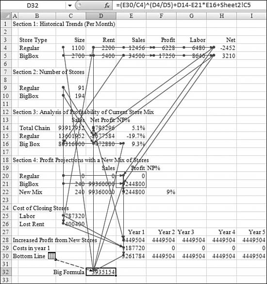
1. From the Formula Auditing group on the Formulas ribbon, click Trace Precedents. Excel draws arrows from the current cell to all the cells that are directly referenced in the formula. In Figure 21.33, for example, an arrow is drawn to a worksheet icon near Cell B30. This indicates that at least one of the precedents for this cell is on another worksheet.

   Figure 21.33. The results of trace precedents for Cell D32.

   

2. Click Trace Precedents again. Excel draws arrows from the precedent cells to the precedents of those cells. These are the second-level precedents of the original cell. Figure 21.34 shows the results of clicking Trace Precedents five times. Practically every cell on the worksheet is a precedent of Cell D32.

   Figure 21.34. Precedents traced five times to find every precedent of the formula.

   

3. To remove the arrows, use the Remove Arrows icon in the Formula Auditing group.

Tracing Dependents

The Formula Auditing section provides another interesting option besides the ones discussed so far in this chapter: You can use it to trace dependents so that you can find all the cells on the current worksheet that depend on the active cell. Before deleting a cell, you might consider clicking Trace Dependents in order to determine whether any cells on the current sheet refer to this cell. This will prevent many #REF! errors from occurring.

Using the Watch Window

If you have a large spreadsheet, you might want to watch the results of some distant cells. You can use the Watch Window icon in the Formula Auditing section of the Formulas ribbon to open a floating box called the Watch Window screen. Here’s what you do:

1. Click the Add Watch icon. The Add Watch dialog appears.
2. In the Add Watch dialog, specify a cell to watch, as shown in Figure 21.35.

   Figure 21.35. Adding a watch to the Watch Window screen.

   

   After you add several cells, the Watch Window screen floats above your worksheet, showing the current value of each cell that was added to it. The Watch Window identifies the current value and the current formula of each watched cell.

In theory, you would use this feature to watch a value in a far-off section of the worksheet.

Evaluating a Formula Slowly

Most of the time, Excel calculates formulas in an instant. It will help your understanding of the formula if you could watch it being calculated in slow motion. If you need to see exactly how a formula is calculated, you can follow these steps:

1. Select the cell that contains the formula you’re interested in.
2. On the Formulas ribbon, in the Formula Auditing group, choose Evaluate Formula. The Evaluate Formula dialog appears, showing the formula. One component of the formula is highlighted: It is the next section of the formula to be calculated.
3. If desired, click Evaluate to calculate the highlighted portion of the formula.
4. Click Step In to begin a new Evaluate section for the cell references in the underlined portion of the formula. Figure 21.36 shows the Evaluate Formula dialog after stepping in to the E30 portion of the formula.

Figure 21.36. The Evaluate Formula dialog allows you to calculate a formula in slow motion.

Evaluating Part of a Formula

Sometimes you do not need to evaluate an entire formula by using the Evaluate Formula feature. In such a case, you can follow these steps:

1. Use the mouse to select just the desired portion of the formula in the formula bar, as shown in Figure 21.37.

   Figure 21.37. You can select a portion of the formula in the formula bar.

   

2. Press F9. Excel calculates just the highlighted portion of the formula, as shown in Figure 21.38.

Figure 21.38. You can press F9 to calculate just the highlighted portion of the formula.