Chapter 22. Understanding Functions

In this chapter

Working with Functions 432

Getting Help with Excel Functions 436

Using AutoSum 438

Using the New General-Purpose Functions in Excel 2007 443

Using the New CUBE Functions in Excel 2007 447

Using the Former ATP Functions 448

The Function Reference Chapters 449

Excel is used on 400 million desktops around the world. People from all careers use Excel, as do many home users who use Excel’s powerful features to track their finances, investments, and more. Part of Excel’s versatility is its wide range of built-in functions.

Excel 2003 offered 255 built-in functions. Another 89 functions shipped with Excel but were available only to people who installed the Analysis Toolpack (ATP). Excel 2007 offers 356 functions. It also includes the following:

• 89 ATP functions, which are now part of the default Excel installation
• 5 new general-purpose functions
• 7 new cube functions that are useful to people who are connecting to a multidimensional database, such as SQL Server Analysis Services

The functions available in Excel 2007 are applicable to a wide range of industries. There are financial functions to help investors, bankers, and bond traders. There are math and statistical functions to help scientists. There are engineering functions for engineers. There are general-purpose functions for everyone. No matter what you are trying to do in Excel, there are functions for you. If there is not a built-in function, there is a good chance that a third-party vendor sells an add-in program to Excel that adds new customized functions to Excel to assist in your particular industry. If not, you can pick up a book on programming VBA to learn how to write your own custom functions in Excel. (For example, Chapter 4 of VBA and Macros for Microsoft Excel by Jelen and Syrstad, offers 30 cool functions you can add to Excel.)

Although it would be impractical to cover each of the 356 functions in great detail in a single chapter, this chapter covers a number of the most commonly used functions in Exce 2007.

Working with Functions

To successfully use functions in a worksheet, you need to follow the function syntax. Keep in mind that a formula that makes use of a function needs to start with an equals sign. You type the function name, an opening parenthesis, function arguments (separated by commas), and the closing parenthesis.

The general syntax of a function looks like this:

=FunctionName(Argument1,Argument2,Argument3)

In general, there should be no spaces anywhere in a function. Specifically, there should never be a space between the function name and the opening parenthesis. Some people like to add a space after each comma in a function, like this:

=FunctionName(Argument1, Argument2, Argument3)

Although this is not required, it does increase the readability of the final function. For what it’s worth, Excel correctly calculates a formula with or without these spaces, so it’s a personal choice as to whether you include them.

Parentheses are needed with every function, including functions that require no arguments. For example, these functions still require the parentheses:

=NOW()
=DATE()

The arguments for a function should be entered in the correct order, as specified in this book or Excel Help. For example, the PMT() function expects the arguments to have the interest rate first, followed by the number of periods, followed by the present value. If you attempt to send the arguments in the wrong order, Excel will happily calculate the wrong result.

In many cases, you can enter arguments as numbers or as cell references. For example, all these formulas are valid:

Excel functions can return a number of errors. This happens most frequently when one of the arguments passed to the function is outside the range of what the function expects. When you receive a #NUM!, #VALUE!, or #N/A! error, you should look in Excel Help for the function. The Remarks section usually indicates exactly what problems can causes each type of error.

The Formulas Ribbon in Excel 2007

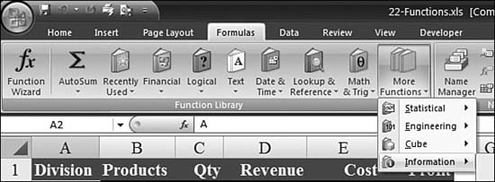
One way to find functions in Excel 2007 is on the Formulas ribbon. The ribbon offers Function Wizard, AutoSum, Recently Used, Financial, Logical, Text, Date & Time, Lookup & Reference, Math & Trig, and More Functions icons.

As shown in Figure 22.1, when you click the More Functions icon, a drop-down with four additional function groups—Statistical, Engineering, Cube, and Information—appears.

Figure 22.1. The Formulas ribbon contains icons for finding functions.

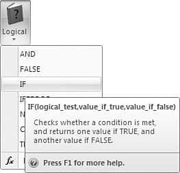
The Formulas ribbon is designed to make it easier to find the right function. You simply select an icon from the ribbon, and an alphabetical list of functions in that group appears. If you hover your mouse over a function in the list, Excel displays a description of what the function does, as shown in Figure 22.2.

Figure 22.2. Hover over a function, and Excel displays a tip, explaining what the function does.

Finding the Function You Need

The inherent problem with the Formulas ribbon is that you often have to guess where your desired function might be hiding. The function categories have been established in Excel for a decade, and in some cases, functions are tucked away in strange places.

For example, the SUM() function is a Math & Trig function. This makes sense because adding numbers is clearly a mathematical process. However, the AVERAGE() function is not available in the Math & Trig icon. (It is under More Functions, Statistical.) The COUNT() function could be math, reference, or information, but it is found under More Functions, Statistical.

By dividing the list of functions up into categories, Microsoft has made it rather difficult to find certain functions. Fortunately, as described in the following sections, there are some tricks you can use to make this process simpler.

Using AutoComplete to Find Functions

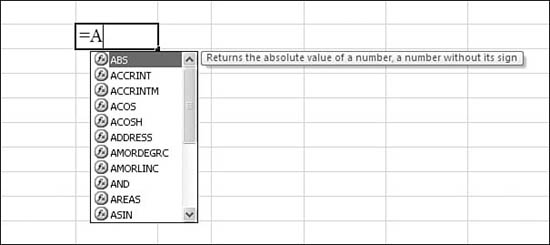
One new feature in Excel 2007 is Formula AutoComplete. Sometimes you might be able to remember the first letter of a function but not all the rest of the letters. For example, there are five varieties of the function you use to do averages, and they all start with A. Rather than trying to figure out whether the averaging function you need is in the Math or Statistical icon, you can just start typing =A in a cell. Excel displays a pop-up window with all the functions that begin with A, as shown in Figure 22.3.

Figure 22.3. Rather than use the icons on the Formulas ribbon, you can type =A to display an alphabetical list of the A functions.

As you continue to type, the pop-up list of functions narrows to a shorter list. After you type =AV, you see a short list of the five averaging functions. You can use the up-arrow and down-arrow keys or the mouse to select a function and read the ToolTip to learn what the function does, as shown in Figure 22.4.

Figure 22.4. As you type a second letter of the function name, you see a shorter list of matching functions. You can use the arrow keys to see a description of what a function does.

To accept a function name from the list, you can either double-click the function name or choose the name and press Tab.

Using the Function Wizard to Find Functions

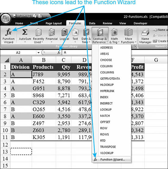
At the bottom of every list of functions is an icon for the Function Wizard. To access the Function Wizard, you can also use the small fx button to the left of the formula bar, or the More Functions option at the bottom of the AutoSum drop-down, or the large Function Wizard button on the Formulas ribbon. Figure 22.5 shows just 3 of the 14 ways you can access the Function Wizard. With 14 different ways to access the Function Wizard, you can guess that this is the best way to find functions.

Figure 22.5. You can access the Function Wizard by using any of these icons.

Choosing any of these options to open the Function Wizard causes the Insert Function dialog to appear.

In the Excel 2003 version of the Function Wizard, Microsoft added a handy search utility. For example, if you typed Car Payment and then clicked Go, Excel would suggest PMT (the correct function) as well as NPER, ISPMT, PV, PPMT, and IPMT. The search functionality was a fantastic addition to Excel 2003 and should be your first stop when trying to find a function in Excel 2007.

When you choose a function in the Insert Function dialog, the dialog displays the syntax for the function, as well as a one-sentence description of the function, as shown in Figure 22.6. If you need more details, you can click the Help on This Function hyperlink in the lower-left corner of the Insert Function dialog.

Figure 22.6. The Insert Function dialog allows you to browse the syntax and descriptions. The Help on This Function hyperlink leads to more help.

Getting Help with Excel Functions

There are three levels of help available for every Excel function: an in-cell ToolTip, the Function Arguments dialog, and Excel Help. You will find the Function Arguments dialog to be one of the best ways of getting help.

Using In-cell ToolTips

In any cell, you can type an equals sign, a function name, and the opening parenthesis. Excel displays a ToolTip that shows the expected arguments. In many cases, this ToolTip is enough to guide you through the function. For example, I can usually remember that the function for figuring out a car loan payment is =PMT(), but I can never remember the order of the arguments. The ToolTip, as shown in Figure 22.7, is enough to remind me that rate comes first, followed by number of periods, and then the principal amount or present value. Any function names displayed in square brackets are optional, so in the example shown in Figure 22.7, you know that you may not have to enter anything for fv or type.

Figure 22.7. The ToolTip will assist you in remembering the proper order for the arguments.

As you type each comma in the function, the next argument in the ToolTip lights up in boldface. This way, you always know which argument you are entering.

Using the Function Arguments Dialog

When you access a function through the Function Wizard or a drop-down list, Excel displays the Function Arguments dialog. This dialog is one of the best features in Excel.

As shown in Figure 22.8, the Function Arguments dialog has many elements:

Figure 22.8. The Function Arguments dialog helps you build a function, one step at a time.

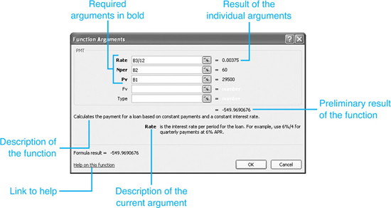
• The one-sentence description of the function appears in the center of the dialog.
• As you tab into the text box for each argument, the description of the argument is shown in the dialog. This description guides you as to what Excel is expecting. For example, in the dialog shown in Figure 22.8, Excel reminds you that the interest rate needs to be divided by four for quarterly payments. This reminds you to divide the APR in Cell B3 by 12.
• To the right of each argument in the dialog is a reference button. You can click this button to collapse the dialog so you can point to the cells for that argument.
• To the right of each text box is a label that shows the result of the entry for that argument.
• Any arguments in bold are required. Arguments not in bold are optional.
• After you enter the required arguments, the dialog shows the preliminary result of the formula. This is on the right side, just below the last argument text box. It appears again in the lower-left corner, just above the Help on This Function hyperlink.
• A Help on This Function hyperlink to the Help topic for the function appears in the lower-left corner of the dialog.

Using Excel Help

The Excel Help topics for the functions are incredibly complete. You will find the following sections in each function’s Help topic:

• The function syntax appears at the top of the topic. This includes a description of each function that may be more complete than the description in the Function Arguments dialog.
• The Remarks section helps troubleshoot possible problems with the function. It discusses specific limits for each argument and describes the meaning of each possible error that could be returned from the function.
• Each function has an example section. You can copy an example to a blank worksheet to see the function actually working.
• The See Also section at the bottom of a Help topic allows you to discover related functions. The logical groupings suggested by See Also is far more useful than the category groupings in the Formulas ribbon.

Figure 22.9 shows the example and See Also sections of a help topic.

Figure 22.9. Excel Help is particularly useful for the Excel functions.

Using AutoSum

Microsoft realizes that the most common function is the SUM() function. It is so popular that Excel provides one-click access to the AutoSum feature.

The AutoSum icon is the large Greek letter sigma that is second icon on the Formulas ribbon. You can click this icon to use AutoSum, or you can use the drop-down at the bottom of the icon to access AutoSum versions of Average, Count Numbers, Max, and Min, as shown in Figure 22.10.

Figure 22.10. The AutoSum drop-down offers the ability to average and more.

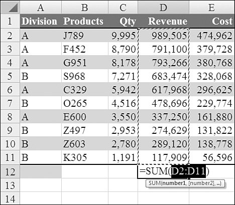
When you click the AutoSum button, Excel seeks to add up the numbers that are above or to the left of the current cell. In general, when you click the AutoSum icon, Excel guesses which cells you are trying to sum. Excel automatically types the SUM() formula. You should review Excel’s guess to make sure that Excel chose the correct range to sum. In Figure 22.11, for example, Excel correctly guesses that you want to sum the column of revenue above the cell.

Figure 22.11. The AutoSum feature is proposing a formula to sum D2:D11.

Potential Problems with AutoSum

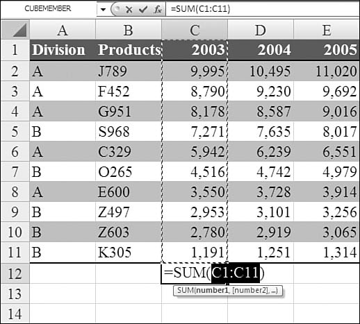
While you should always check the range proposed by the AutoSum feature, there are some cases in which you should be especially wary. If your headings above the data are numeric, for example, this will fool AutoSum. In Figure 22.12, the 2003 heading in C1 is numeric. This causes Excel to incorrectly include the heading in the total for Column C.

Figure 22.12. Numeric headings confuse AutoSum.

When Excel proposes the wrong range for a sum, you use your mouse to highlight the correct range before pressing Enter.

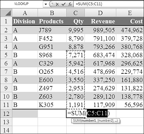
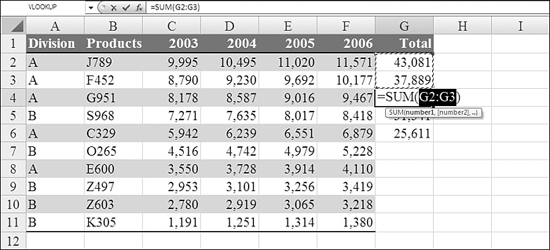
Excel avoids including other SUM() functions in an AutoSum range. If a range contains a SUM() function that references other cells, Excel prematurely stops just before the SUM() function. In Figure 22.13, Cell C4 contains the formula =SUM(H3:H4). Using AutoSum in Cell C12 causes Excel to propose summing C5:C11. This problem happens only when the SUM() function references other cells. If Cell C4 contained =7000+1878 or =H3+H4 or =SUM(7000,1878), AutoSum would include the cell.

Figure 22.13. A SUM() function like the one in Cell C4 causes AutoSum to stop prematurely.

Excel prefers to sum a column of numbers instead of a row of numbers. Figure 22.14 shows a strange anomaly. If you place the cell pointer in Cell G2 and click AutoSum, Excel correctly guesses that you want to total C2:F2. Cell G3 works fine. However, when you get to Cell G4, Excel has a choice. There are two numbers above G4 and four numbers to the left of G4. Because there are two numbers directly above, Excel tries to total those two numbers. This problem only seems to happen in the third row of the dataset. After that, Excel sees that the three cells above are all summing across the rows, and AutoSum works perfectly in G5:G11.

Figure 22.14. Excel can choose between summing two numbers above or four numbers to the left. Excel chooses incorrectly.

Special Tricks with AutoSum

There is an amazing trick you can use with AutoSum. If you select a range of cells before clicking the AutoSum button, Excel does a much better job of predicting what to sum.

In Figure 23.13, for example, you could select G2:G11 before clicking the AutoSum button, and Excel would know to sum each row. Be careful, though, because Excel does not preview its guess before entering the formula. You should always check a formula after using AutoSum to make sure the correct range was selected.

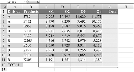
If your selection contains a mix of blank cells and nonblank cells, Excel adds the AutoSum to only the blank cells. In Figure 22.14, for example, you select the range C1:G12 before clicking the AutoSum button.

Figure 22.15. If your selection contains a mix of blank and nonblank cells, AutoSum only writes to the blank cells.

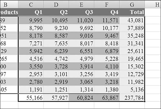
After you click the AutoSum button, Excel correctly filled in totals for all the rows and columns, as shown in Figure 22.16.

Figure 22.16. By using AutoSum, you can add 15 SUM() formulas with one click.

Using the AutoSum Drop-Down

In prior versions of Excel, the AutoSum button was flanked by a small drop-down arrow that allowed you to use the AutoAverage, AutoMin, AutoMax, and AutoCount features. In Excel 2007, you can still click an arrow to access these features, and the drop-down arrow on the icon is more prominent than it used to be.

To see how this works, you can select a cell or range of cells. From the AutoSum drop-down, you choose another function. Excel uses the same guessing logic as with AutoSum, but it instead enters a formula for Average, Min, Max, or Count, as shown in Figure 22.17.

Figure 22.17. You can use the drop-down on the AutoSum icon to access the features AutoAverage, AutoMin, AutoMax, and AutoCount.

Using the New General-Purpose Functions in Excel 2007

Excel 2007 has five new functions that were added at the request of customers: IFERROR(), AVERAGEIF(), SUMIFS(), AVERAGEIFS(), and COUNTIFS(). As described in the following sections, they are a great addition to the Excel function set.

The Best New Addition: IFERROR()

Excel errors are not the friendliest things. No one really understands the screaming #VALUE! or #N/A! errors. With the all-capital letters and the exclamation point, they are scary looking. Furthermore, the default performance is that one single #N/A error in a column of one million good values causes the total for the column to calculate as #N/A.

In Chapter 24, “Using Powerful Functions: Logical, Lookup, and Database Functions,” you will learn about the VLOOKUP() function. The VLOOKUP() function is great, for example, for converting a number to a name. Say that your company hires a new employee and you encounter data for the employee before anyone has updated the lookup table. This results in an #N/A! error.

You might want the table to include something friendlier than the #N/A! error. Perhaps you would like the text New Rep to appear instead of the unfriendly #N/A!. There was not an easy way to do this in prior versions of Excel. You had to use a formula such as =IF(ISNA(VLOOKUP(A2,$AA$1:$AB$99,2,FALSE)), "New Rep", VLOOKUP(A2,$AA$1:$AB$99,2,FALSE)). This formula forces Excel to use the VLOOKUP() function once, determine if it is an #N/A error, and then calculate the VLOOKUP() function again. This is a pain for anyone using Excel. If they have to change the VLOOKUP(), they have to change it twice in the formula. Also, it takes Excel longer to calculate because it potentially has to do each good VLOOKUP() twice.

Microsoft corrected this problem in Excel 2007 by adding the IFERROR() function. With the IFERROR() function, you can use VLOOKUP() function once and then provide an alternate value or formula in case the VLOOKUP() function returns an error.

The following section describes using IFERROR().

Syntax: IFERROR(valueM,value_if_error)

This function returns a value you specify if a formula evaluates to an error; otherwise, it returns the result of the formula. You use the IFERROR() function to trap and handle errors in a formula.

Note the following in this syntax:

• value is the value, cell reference, or formula that is checked for an error.
• value_if_error is the value to return if the formula evaluates to an error.
• The following error types are evaluated: #N/A, #VALUE!, #REF!, #DIV/0!, #NUM!, #NAME?, and #NULL!.
• If value or value_if_error is an empty cell, IFERROR() treats it as an empty string value (that is, "").
• If value is an array formula, IFERROR() returns an array of results for each cell in the range specified in value.
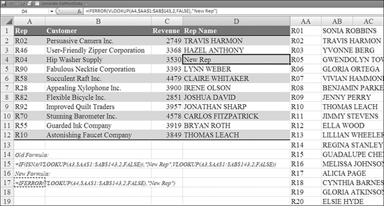
• In this example, the long formula with two VLOOKUP() functions is shortened to =IFERROR(VLOOKUP(A2,$AA$1:$AB$99,2,FALSE), "New Rep"). As you can see, using the IFERROR() function is much easier and faster.

Figure 22.18 shows the IFERROR() function.

Figure 22.18. You can use the IFERROR() function to capture #N/A! errors in VLOOKUP() errors, divide-by-zero errors, or any other errors you can foresee.

Adding AVERAGEIF() to Conditional Formulas

COUNTIF() and SUMIF() have been a part of Excel for several years. These functions allow you to calculate a total for records in a range that match one particular condition. Although you could always do this with an array formula, people have found SUMIF() and COUNTIF() to be easier to use.

Microsoft has added AVERAGEIF() to the function list. This function, which is similar to SUMIF(), is described in the following section.

Syntax: AVERAGEIF(range,criteria,[average_range])

This function returns the average (arithmetic mean) of all the cells in a range that meet a given criterion.

Note the following in this syntax:

• range is one or more cells to average.
• criteria is the criteria in the form of a number, an expression, a cell reference, or text that defines which cells are averaged. For example, criteria can be expressed as 32, "32", ">32", "apples", or B4.
• average_range is the set of cells to average. If this is omitted, range is used.
• Cells in range that contain TRUE or FALSE are ignored. If a cell in range or average_range is an empty cell, AVERAGEIF() ignores it. If a cell in criteria is empty, AVERAGEIF() treats it as a 0 value. If no cells in the range meet criteria, AVERAGEIF() returns the #DIV/0! error value.
• You can use the wildcard characters question mark (?) and asterisk (*) in criteria. A question mark matches any single character; an asterisk matches any sequence of characters. If you want to find an actual question mark or asterisk, you need to type a tilde (~) before the character.
• average_range does not have to be the same size and shape as range. Which cells are averaged is determined by using the top-left cell in average_range as the beginning cell and then including cells that correspond in size and shape to range.

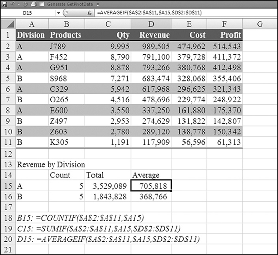
In Figure 22.19, the formulas in D15:D16 use the AVERAGEIF() formula to average only the records that match the divisions in A15:A16.

Figure 22.19. Like SUMIF() and COUNTIF(), the new AVERAGEIF() function can filter records based on one criterion.

Using Conditional Formulas with Multiple Conditions: SUMIFS(), AVERAGEIFS(), and COUNTIFS()

When someone sees how easy using SUMIF() is, and they invariably want the function to do more. One of the most frequent questions at the MrExcel message board is along the lines of this: “I am using SUMIF() to get a total by region. How can I put two conditions in there to only get the total for a certain region and product?” In versions of Excel prior to Excel 2007, there were ways to do this, but they were difficult. You had to use either SUMPRODUCT() or an array formula. There is a lot of complexity in going from a simple SUMIF() to the complex Boolean logic required to understand SUMPRODUCT().

Thankfully, in Excel 2007, Microsoft implemented new versions of SUMIF(), COUNTIF(), and AVERAGEIF() that can handle not just two conditions, but unlimited conditions. The three new functions add the letter S to the end of the function name (that is, SUMIFS(), COUNTIFS(), and AVERAGEIFS()), to signify that multiple IFs are being considered. With SUMIFS() and AVERAGEIFS(), you first specify the range to be summed or averaged. You then specify pairs of arguments. In each pair, you first specify the range to check and then the value to match in that range. The following sections describe these three functions.

Syntax: SUMIFS(sum_range,criteria_range1,criteria1[,criteria_range2,criteria2...] )

The SUMIFS() function adds the cells in a range that meet multiple criteria.

Note the following in this syntax:

• sum_range is the range to sum.
• criteria_range1, criteria_range2, and so on are one or more ranges in which to evaluate the associated criteria.
• criteria1, criteria2, and so on are one or more criteria in the form of a number, an expression, a cell reference, or text that define which cells will be added. For example, they can be expressed as 32, "32", ">32", "apples", or B4.
• Each cell in sum_range is summed only if all the corresponding criteria specified are true for that cell.
• Cells in sum_range that contain TRUE evaluate to 1; cells in sum_range that contain FALSE evaluate to 0.
• You can use the wildcard characters question mark (?) and asterisk (*) in criteria. A question mark matches any single character; an asterisk matches any sequence of characters. If you want to find an actual question mark or asterisk, you need to type a tilde (~) before the character.
• Each criteria_range does not have to be the same size and shape as sum_range. Which cells are averaged is determined by using the top-left cell in that criteria_range as the beginning cell and then including cells that correspond in size and shape to sum_range.

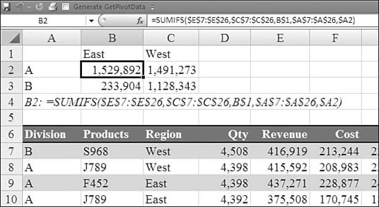
In Figure 22.20, you want to build a table that shows the total by region and product. sum_range is the revenue in E7:E26. The first criteria pair consists of the regions in $C$7:$C$26 being compared to the word East in B$1. The second criteria pair consists of the divisions in $A$7:$A$26 being compared to the letter A in $A2. The formula in B2 is =SUMIFS($E$7:$E$26,$C$7:$C$26,B$1,$A$7:$A$26,$A2). You can copy this formula to B2:C3.

Figure 22.20. The new SUMIFS() function is used to create this summary by region and product.

Syntax: AVERAGEIFS(average_range,criteria_range1,criteria1[,criteria_range2,criteria2...])

The AVERAGEIFS() function is similar to SUMIFS(). It returns the average (arithmetic mean) of all cells that meet multiple criteria. The arguments are the same as for SUMIFS().

Syntax: COUNTIFS(range1,criteria1[,range2, criteria2...])

COUNTIFS() counts the number of cells in a range that meet multiple criteria. The COUNTIFS() syntax is a bit different from the syntax of the other new functions. With COUNTIFS(), there is no need to specify sum_range. The arguments in COUNTIFS() consist of pairs specifying criteria. The first argument in each pair specifies a criteria region. The second argument in each pair specifies the criteria value to match.

Using the New CUBE Functions in Excel 2007

Several high-end analysis tools store data in a multidimensional format. Examples of these services are Essbase and SQL Server Analysis Services.

With Microsoft’s increased focus on business intelligence, they are encouraging more large businesses to purchase SQL Server Analysis Services from Microsoft. To assist those customers, the new CUBE functions help these customers extract data from their databases.

In most cases, you will never actually enter these functions. They are created for you automatically after you (1) build a pivot table based on an OLAP data source and (2) choose Pivot Table Tools, Options, OLAP Tools, Convert to Formulas to convert the pivot table to live formulas. In response, Excel will automatically enter the proper cube functions.

Excel automatically creates formulas for you, using the seven new cube functions. Most of the time, you encounter these formulas after they have been created for you by Excel.

While 99% of Excel customers will never need these formulas, and 99% of the remaining 1% will have Excel create the formulas automatically, it is possible to write the formulas manually. You have to specify the connection string to identify the OLAP source.

The following sections provide a brief overview of the cube functions. If you need to create these formulas manually, consult Excel help for more details.

Syntax: CUBEMEMBER(connection,member_expression[,caption])

The CUBEMEMBER() function returns a member or tuple in a cube hierarchy. You can use it to validate that the member or tuple exists in the cube.

Syntax: CUBEMEMBERPROPERTY(connection,member_expression,property)

The CUBEMEMBERPROPERTY() function returns the value of a member property in the cube. You can use it to validate that a member name exists within the cube and to return the specified property for that member.

Syntax: CUBERANKEDMEMBER(connection,set_expression,rank[,caption])

The CUBERANKEDMEMBER() function returns the nth, or ranked, member in a set. You can use it to return one or more elements in a set, such as the top sales performer or top 10 students.

Syntax: CUBESET(connection,set_expression[,caption][,sort_order][,sort_by])

The CUBESET() function defines a calculated set of members or tuples by sending a set expression to the cube on the server, which creates the set. The function then returns that set to Excel. You can use CUBESET() to build dynamic reports that aggregate and filter data, by using the return value as a slicer in the CUBEVALUE() function, the CUBERANKEDMEMBER() function to choose specific members from the calculated set, and the CUBESETCOUNT() function to control the size of the set.

Syntax: CUBESETCOUNT(set)

The CUBESETCOUNT() function returns the number of items in a set.

Syntax: CUBEVALUE(connection,member_expression1[,member_expression2...])

The CUBEVALUE() function returns an aggregated value from a cube.

Syntax: CUBEKPIMEMBER(connection,kpi_name,kpi_property[,caption])

The CUBEKPIMEMBER() function returns a key performance indicator (KPI) name, property, and measure, and it displays the name and property in the cell. A KPI is a quantifiable measurement, such as monthly gross profit or quarterly employee turnover, used to monitor an organization’s performance. (To use this function, you must have SQL Server Analysis Services 2005 or later.)

Using the Former ATP Functions

In versions of Excel prior to Excel 2007, a wide variety of functions were known as the ATP functions. These functions were available only on computers that had enabled the Analysis Toolpack (ATP) add-in.

Even if you had enabled the ATP, there was a danger that you could send a workbook to a co-worker who had not enabled the ATP. If this happened, all the formulas that used any of the 89 ATP functions would change to NAME! errors.

Although it was easy to enable the ATP (by selecting Tools, Add-ins, Check Analysis Toolpack and then clicking OK), there was a great deal of paranoia about using these functions, sending the workbook out, and having others obtain the wrong results. For this reason, some companies instituted policies against using the ATP functions. People would write elaborate formulas to duplicate what could easily be done with the ATP.

In a smart move, Microsoft has promoted the 89 ATP functions to be part of the standard Excel package starting with Excel 2007. This means that you can safely share an Excel 2007 workbook with any other person using Excel 2007, and all the functions will continue to work. However, you need to be aware that if you are sharing a workbook with a person who is using a legacy version of Excel, the functions in the ATP may change to NAME! errors on the other computer.

The individual functions are covered in the next five chapters. However, the following alphabetical list is provided as a guide to which functions are potentially problems when sharing with people using prior versions of Excel.

The following are the functions that used to be included in the ATP but are now a default part of Excel 2007: ACCRINT(), ACCRINTM(), AMORDEGRC(), AMORLINC(), BESSELI(), BESSELJ(), BESSELK(), BESSELY(), BIN2DEC(), BIN2HEX(), BIN2OCT(), COMPLEX(), CONVERT(), COUPDAYBS(), COUPDAYS(), COUPDAYSNC(), COUPNCD(), COUPNUM(), COUPPCD(), CUMIPMT(), CUMPRINC(), DEC2BIN(), DEC2HEX(), DEC2OCT(), DELTA(), DISC(), DOLLARDE(), DOLLARFR(), DURATION(), EDATE(), EFFECT(), EOMONTH(), ERF(), ERFC(), ERROR.TYPE(), FACTDOUBLE(), FVSCHEDULE(), GCD(), GESTEP(), HEX2BIN(), HEX2DEC(), HEX2OCT(), IMABS(), IMAGINARY(), IMARGUMENT(), IMCONJUGATE(), IMCOS(), IMDIV(), IMEXP(), IMLN(), IMLOG10(), IMLOG2(), IMPOWER(), IMPRODUCT(), IMREAL(), IMSIN(), IMSQRT(), IMSUB(), IMSUM(), INTRATE(), ISEVEN(), ISODD(), LCM(), MDURATION(), MROUND(), MULTINOMIAL(), NETWORKDAYS(), NOMINAL(), OCT2BIN(), OCT2DEC(), ODDFPRICE(), ODDFYIELD(), ODDLPRICE(), ODDLYIELD(), PRICE(), PRICEDISC(), PRICEMAT(), QUOTIENT(), RANDBETWEEN(), RECEIVED(), SERIESSUM(), SQL.REQUEST(), SQRTPI(), TBILLEQ(), TBILLPRICE(), TBILLYIELD(), WEEKNUM(), WORKDAY(), XIRR(), XNPV(), YEARFRAC(), YIELD(), YIELDDISC(), YIELDMAT().

The Function Reference Chapters

The next five chapters provide a fairly comprehensive reference for most of the 356 functions in Excel 2007. At the beginning of each of these chapters is an alphabetical list of the functions described, along with arguments and a short description of each function. Following the alphabetical list are examples of how to use the functions. These examples describe all the required arguments. The examples are designed to give you ideas of how to use the functions in real life.

Function coverage is broken out as follows:

• Chapter 23, “Using Everyday Functions: Basic Math and Date Functions,” describes functions that many people encounter in their everyday life: some of the math functions, date functions, and text functions.
• Chapter 24, “Using Powerful Functions: Logical, Lookup, and Info Functions,” describes functions that are a bit more difficult but that should be a part of your everyday arsenal. These include a series of functions for making decisions in a formula. They include the IF function and are known collectively as the logical functions. Chapter 24 also describes the information, lookup, and database functions.
• Chapter 25, “Using Financial Functions,” describes the financial functions. The first section of the chapter includes functions that anyone can use to calculate a car loan or to plan for retirement. The later sections of the chapter include functions for depreciation, business valuation, and bond investing.
• Chapter 26, “Using Statistical Functions,” describes statistical functions. Many of these functions are functions that are useful everyday (for example, AVERAGE(), MAX(), MIN(), RANK()). The chapter also describes many highly specialized functions that are useful to scientists and engineers.
• Chapter 27, “Using Math and Engineering Functions,” describes trigonometry and engineering functions. The trigonometry functions are grouped along with the other math functions in the Math Functions icon, but they are described separately in this book because they are more specialized. The engineering functions are highly specialized.