Chapter 12. Pivot Table Data Crunching for Excel 2007

In this chapter

Grouping Daily Dates to Months and Years 238

Sorting and Filtering 239

Exploring Even More Filtering Options 246

Adding New Items Along a Dimension 255

Showing Percentages Instead of Values 258

Exploring Interesting Uses for Pivot Tables 263

Finding More Information on Pivot Tables 269

Pivot tables in Excel 2007 offer far more options than what have been discussed in the previous two chapters. This chapter will show you how to expand the possibilities of analyses available with pivot tables. This is a great sampling of the most common analyses you might want to perform. If you want to see every possible feature in a pivot table, check out the Pivot Table Data Crunching book that Mike Alexander and I wrote. It is available from the Que Business Solutions series.

Grouping Daily Dates to Months and Years

In Chapter 10, I encouraged you to go back to your source software and ask for a report of data at the detail level. This data will undoubtedly report data at the daily level instead of the monthly level.

People in manufacturing plants care about the productivity from every day. However, people in accounting tend to care about performance of each month.

Pivot tables make it incredibly easy to roll data up from daily dates to weekly, monthly, quarterly, or yearly analyses, depending on your requirements.

The best way to teach you this technique is to walk through a real example. Of course, in your data, fields might be slightly different. Let’s assume, though, that you have some sort of field with data at the daily level.

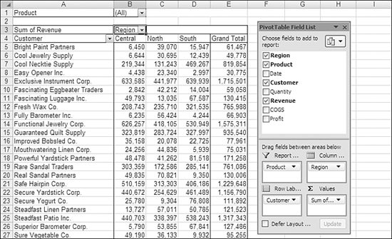
The pivot table in Figure 12.1 has three fields in the Row Labels section, and it has the Date field in the Column Labels section. Because the original data on which this pivot table is based had information by day, the pivot table has 471 columns, which is not very useful.

Figure 12.1. Because the underlying transactional date had daily dates, a summary pivot table by date starts out showing daily dates.

Notice in the Group section of the Options ribbon that Group Field is grayed out. Now look to the right, in the Active Field section. Currently, the active field is the Region field, probably because the cell pointer is currently on a Region field in Cell A5.

If you use the cell pointer to select a date in Cell B4, the Active Field section changes to show that Date is the active field. The Group Field icon becomes active. You can click the Group Field icon to display the Grouping dialog box, which is shown in Figure 12.2.

Figure 12.2. Choose to group by Months and Years

In the Grouping dialog, be sure to choose both Months and Years, as shown in Figure 12.2. You can also group by quarters.

After you select Months and Years, the daily dates along the top of the pivot table are replaced with months. In the PivotTable Field List box, there are now two fields in the Column Labels layout section: The Date field now contains your monthly data, and a new virtual field called Years is added to the list.

Sorting and Filtering

The ability to filter data has improved dramatically in Excel 2007. Few people were able to locate the Top 10 AutoShow settings in previous versions of Excel, but they are now much easier to access—right from the PivotTable Field List box.

In case you never encountered the Top 10 AutoShow in previous versions of Excel, it would allow you to limit a report to show the top 15 customers or the bottom 5 products.

My general rule is that the higher the manager, the less they can deal with detailed data. The new Filtering features in Excel 2007 pivot tables will let you limit the report to just the top n records.

In Excel 2007, this feature is easier to access from the PivotTable Field List box. Being able to produce a report of the top n items makes pivot tables even more powerful.

The following examples walk through a sample dataset. In your dataset, you can easily extrapolate to achieve a similar result for any field.

Figure 12.3 shows a pivot table that lists revenue by customer for two years. There are 30 different customers in the list. Customers are listed down the row area, and the Years field goes across the column area. Revenue for the two years totals $13.3 million.

Figure 12.3. This pivot table showing revenue by customer is unfiltered and unsorted.

You can access Excel’s powerful filtering and sorting features for any field in the field list portion of the PivotTable Field List box. In Figure 12.4, Customer appears twice in the PivotTable Field List box. The Customer field visible in the Row Labels layout section already has a drop-down visible. This is not the field you want to use. You therefore need to hover over the Customer field that appears in the top portion of Figure 12.4. When you hover over any field in the field list, a drop-down appears near the field, as shown in Figure 12.4.

Figure 12.4. You hover over any field in the field list and then choose the drop-down arrow that appears.

Limiting a Report to the Top Seven Customers

Sales managers often like to see reports of the top customers. Pivot tables enable you to easily create such reports.

To create a report of a company’s top customers, you hover over the Customer field in the field list portion of the PivotTable Field List box. When a drop-down appears near the list, you should choose it. You want to filter the list based on a value in the table, so you should choose the Value Filters selection. As shown in Figure 12.5, the final choice in the Value Filters is Top 10. You should choose this option.

Figure 12.5. To find the customers with top revenue, you can filter on customer.

Excel displays the Top 10 Filter dialog for the Customer field. Initially, this dialog offers to display the top 10 items, by sum of revenue. You can change the dialog to show the top or bottom customers, and you can change it to display any number of items. Figure 12.6 shows a report of the top seven customers.

Figure 12.6. A company’s top seven customers, determined using the Top 10 Filter on the Customer field.

Showing the Bottom 25% of Customers

In the previous example, you asked for a specific number of customers or products or items. Although this feature is often called the top 10 feature, it can be used to show either the top or bottom of the dataset. It can be used to show n items, or the items that make up n% of the dataset.

If your company has 12 customers, showing the top 10 customers will not be that interesting. Futher, if your company has 12,000 customers, showing the top 10 might miss a lot of customers.

The following example walks through how to limit the report to a percentage of the customers.

To show the bottom quarter of customers, you can use the Value filter in the Customer drop-down to select the Top 10 filter again. This time, however, you choose Bottom 25 Percent based on Sum of Revenue. Figure 12.7 shows the result of doing this.

Figure 12.7. These 23 customers comprise the bottom 25% of a company’s revenue.

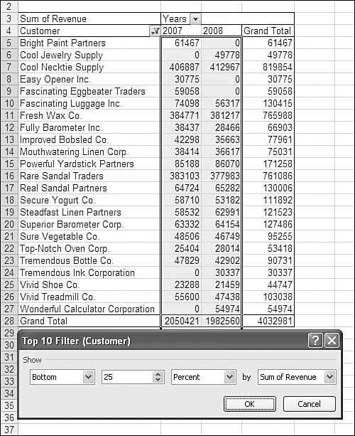
The original dataset had $13.3 million of revenue. Twenty-five percent of $13.3 million is $3.3 million. Curiously, applying the Bottom 25 Percent filter results in 23 customers and $4 million of revenue. This initially does not make sense: $4 million is 30% of the revenue coming from 77% of your customers. The largest value in Figure 12.7 is Cool Necktie Supply, at $819,000. If Excel would have excluded this customer, the report would have contained only $3.2 million of revenue. Because that is just short of 25%, Excel includes the next smallest customer to make sure you see at least 25% of the revenue.

Showing the Top or Bottom Customers Who Make Up a Specific Dollar Amount

The Top 10 Filter dialog offers a new and interesting third option. Instead of asking for items or a percentage, you can ask for a particular sum, as shown in Figure 12.8.

Figure 12.8. The Sum function is new in the Top 10 Filter dialog.

You can ask to see the customers who make up the bottom $1.5 million. However, the spin button paradigm clearly does not work here. It would literally take 1,499,989 clicks on the up spin button. You could attempt to use the spin button in Figure 12.8 to dial up to 1,500,000, but it would take forever. When you want to use the Sum function, you can actually click into the second field in the dialog and type a number such as 1500000.

The result shown in Figure 12.9 includes enough customers so that the total exceeds $1.5 million. Fascinating Luggage in Row 9 pushes the total over $1.5 million, to end at $1,514,795.

Figure 12.9. The third option in the Top 10 Filter dialog locates the customers who account for a specific amount of revenue.

Sorting a Field

In Figures 12.3 through 12.9, the filtered pivot table report is presented in alphabetical order. In each case, the report would be more interesting if it were presented sorted by revenue instead of by customer name.

The Customer drop-down offers choices to sort a field in ascending or descending order, as shown in Figure 12.10. However, you can find more powerful options by selecting More Sort Options from this drop-down.

Figure 12.10. The Customer drop-down shows choices to sort alphabetically, but the real power is behind the More Sort Options choice.

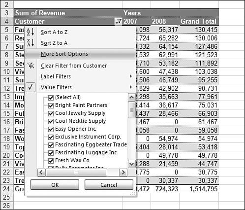
When you choose More Sort Options from the Customer drop-down, the Sort dialog appears. This dialog initially offers to sort in ascending order, based on customer. If you choose Descending and then use the drop-down, you can choose to sort the report based on sum of revenue. This produces the report shown in Figure 12.11.

Figure 12.11. To create a report sorted from high to low by revenue, choose to sort the customer field based on sum of revenue.

Take a look at the report in Figure 12.11. Note that it is sorted based on grand total revenue. What if you wanted to sort the report based on 2007 revenue? Excel 2007 now gives you the capability to do this. After choosing More Sort Options, you click the More Options button in the Sort dialog to open the More Sort Options dialog.

As shown in Figure 12.12, the More Sort Options dialog includes a section to sort by the grand total. If you change this option to Sort by Values in Selected Row, you can then specify that the customer sort should be based on either Column B or Column C. In Figure 12.12, Values in Selected Row is set to $B$5 to indicate that the report should be sorted by 2007 revenue. The left side of Figure 12.12 shows the result of this sort.

Figure 12.12. Perhaps this dialog should be called Even More Sort Options or Double Super Secret Sort Options.

Why Not Sort with the Data Ribbon?

You might be wondering why you should go to the hassle of using the Sort and More Sort Options dialogs. Wouldn’t it be easier to select Cell B5 and use the Sort Descending button on the Data ribbon? Yes. It would be easier to sort by clicking this button for this one view of the pivot table. However, as you continue to pivot the table into other configurations, Excel does not remember that you always want the data sorted into this particular sort. If you use the sort options in the PivotTable Field List box, you are telling Excel to always sort this pivot table in a certain way. Any sort property you set here will remain in effect as you add and remove fields.

Figure 12.13 shows the same table from Figure 12.12, with the Customer filter removed. Because the report is sorted based on the Customer field, Excel continues to sort the report in descending revenue order from 2007.

Figure 12.13. This interesting view makes you wonder why you lost Bright Paint as a customer in 2008.

Exploring Even More Filtering Options

The Top 10 Value filter has been around for years. Excel 2007 introduces all sorts of interesting filters. For example, Figure 12.14 shows the options available to filter the Customer field based on the labels in the Customer column.

Figure 12.14. This list shows the ways to filter the Customer field based on the labels in the customer column.

If your team is assigned customers alphabetically, you can ask for just the customers between A and E. You can ask for just customers with a particular word in their name. You can ask for customers that end in Inc. You can filter based on literally anything. Figure 12.15 shows the Label Filter dialog, where you can select numerous filters.

Figure 12.15. One of the myriad label filters available.

Filtering Using Check Boxes

The Customer drop-down includes a list of all the customers in the database. If you needed to exclude a few specific customers, you could simply uncheck their boxes in the filter list, as shown in Figure 12.16.

Figure 12.16. Based on Figure 12.14, you know that three customers had no revenue in 2008. The filter shown here removes those three customers from the analysis.

Because it is easier to select 3 customers than to unselect 27, if you need to remove most of the items from the list of customers, you can follow these steps:

1. Choose Select All to reselect all customers.
2. Choose Select All to uncheck all customers.
3. Select the particular customers you want to view.

The results are shown in Figure 12.17.

Figure 12.17. You can turn Select All on and then off to unselect all customers.

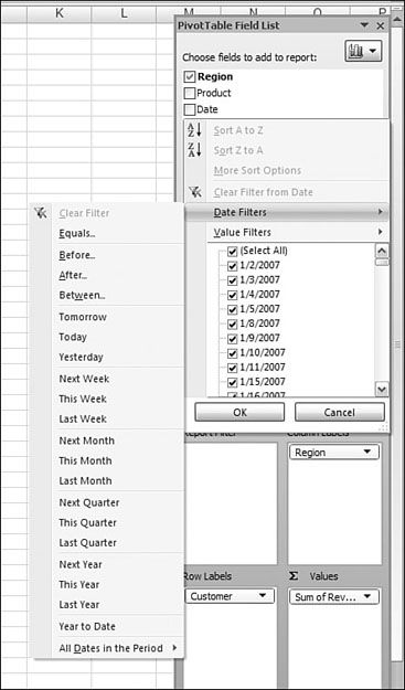
Using Date Filters

It is possible to sort by fields that are not currently displayed in a pivot table. Figure 12.18 shows a variety of date filters that are available for the Date field. In addition to the standard filters, such as This Year, Next Year, and Last Year, the report offers powerful filters such as Year to Date.

Figure 12.18. Excel offers a number of canned date filters. Users of QuickBooks will recognize this list.

As an example of using a date filter, Figure 12.19 shows all dates in the period Quarter 4.

Figure 12.19. All dates in Quarter 4.

Filtering by Using the Report Filter

Those who are familiar with pivot tables in previous versions of Excel know the report filter as the Page Field area of the layout. Although the new field filtering tools described in the preceding sections offer far more powerful filtering, you can use the report filter drop zone to add filter cells to a pivot table in order to do basic ad hoc analysis.

To add a filter dropdown to the top of the pivot table, you drag the Product field to the Report Filter section of the PivotTable Field List box, as shown in Figure 12.20. This adds a new heading called Product in Cell A1. Cell B1 then contains a drop-down that is initially set to (All).

Figure 12.20. The Product field is added as a report filter.

Next, from the drop-down in Cell A2, you need to select a product from the list. The pivot table then redraws, showing only totals for that product (see Figure 12.21). This is a great report to give to a marketing manager for product G101.

Figure 12.21. A report for a single product.

Excel 2007 now gives you the ability to choose multiple items in the report filter. The Product drop-down contains the Select Multiple Items check box. If you choose this option, each product in the list is prefixed by a check box. You can select multiple items for the filter, as shown in Figure 12.22.

Figure 12.22. You can now select multiple items from the filter drop-down.

Looping Through Each Value in a Report Filter

With the report filter, it is easy to print a report for one specific product or region or any field.

After you print a report for the manager interested in that one specific item, word will spread, and all the other managers will want the similar report. Selecting each value one at a time can get tedious. Creating a tiny Excel VBA macro can simplify the process. The following macro will print the pivot table for each value found in the product report filter:

For more information on macros, see Chapter 36, “Automating Repetitive Functions Using VBA Macros.”

Using Show Pages to Replicate a Pivot Table

While this previous macro will print many versions of one pivot table, there is an alternate solution to the problem. This technique actually makes many copies of the pivot table, with a different Report Filter value in each copy. If your pivot table contains at least one Report Filter field, select the Options dropdown from the Options ribbon. Choose Show Pages from the dropdown menu. Confirm which field should be used. Excel will add worksheets to your workbook. Each worksheet will contain the original pivot table, with a different value chosen for the selected filter field.

Building the Ultimate Ad Hoc Reporting Tool

The report filter is a great ad hoc answer tool. You could, in theory, give a pivot table with multiple report filters to your VP and allow him to answer many questions that might arise. This type of report allows for ad-hoc querying of the underlying data.

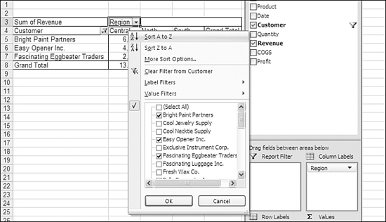
To build an ad-hoc query report, you move all your label fields to the report filter area. You also move all the value fields to the Σ Values area, as shown in Figure 12.23.

Figure 12.23. An ad hoc reporting tool.

If someone calls with a question, such as these, you can quickly find the answer by using the various drop-downs:

• How much did we sell in the north region? (Figure 12.24 shows how to answer this question.)

Figure 12.24. North region sales.

• How much did the Fresh Wax customer buy? (Figure 12.25 shows how to answer this question.)

Figure 12.25. Sales to Fresh Wax.

• How many of product A354 did the south region sell in January 2007? (Figure 12.26 shows how to answer this question.)

Figure 12.26. Sales of A354 in the south region.

Using a Formula to Add a Field to a Pivot Table

In the examples shown in the preceding sections, the pivot table shows all the value fields from the original dataset. In some cases, however, you might want to add new fields, such as Average Price or Gross Profit Percent. You can add new fields by using the Calculated Field tool.

Select PivotTable Tools, Options, Tools, Formulas, Calculated Field.... This will display the Insert Calculated Field dialog, as shown in Figure 12.27.

Figure 12.27. You use this dialog to define a calculated field.

To add a field to the pivot table, you follow these steps:

1. In the Insert Calculated Field dialog, first type a name for the field. The field name should not contain spaces. In this particular example, a name such as GPPct (for Gross Profit Percent) would work.
2. Build your formula using the field names in the Fields listbox and the Insert Field button. In this example, the formula for determining gross profit percent is profit divided by revenue, so click Profit in the Fields list and then click Insert Field.
3. Type a slash (/) to indicate division.
4. Click Revenue in the Fields list and then click Insert Field. The dialog now looks as shown in Figure 12.28.

   Figure 12.28. Defining a Gross Profit Percent calculated field.

   

5. Click the Add button to accept the GPPct field.
6. You can define additional fields as needed. For example, enter AveragePrice in the Name text box to add another field.
7. The formula for average price is revenue divided by quantity, so select the Revenue field and then click Insert Field.
8. Type a slash (/) to indicate division.
9. Select the Quantity field and then click Insert Field.
10. Click OK to close the dialog.
11. The fields are added to the pivot table as Sum of GPPct and Sum of AveragePrice. Both fields have numeric formatting that is inappropriate, as shown in Figure 12.29.

    Figure 12.29. The calculations are correct, but the numeric formatting is wrong.

    

12. Select Sum of GPPct in Cell E7. Then, in the Active Field group, choose Field Settings to display the Data Field Settings dialog for the field.
13. In the Custom Name box, type a new name for the field. The current name of Sum of GPPct is not correct. Excel calculates the formula on the totals, so it is really a Gross Profit Percent of the Sums, but this is not a very good name. You might be tempted to use GPPct again, but you must change the name slightly here, as shown in Figure 12.30.

    Figure 12.30. Adjust the name and numeric formatting in the Data Field Settings dialog.

    

14. In the Data Field Settings dialog, click the Number Format button. Assign a numeric format of Percentage with one decimal place.
15. Repeat steps 12–14 for the AveragePrice field, assigning to it a numeric format of Currency with two decimal places.

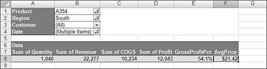
After you correctly define the fields, they are correctly calculated for any variation of the pivot table. Figure 12.31 shows details for sales of Item A354 by month. This report shows a fair amount of variability in pricing from month to month.

Figure 12.31. The calculated fields apply to any combination of label fields.

Adding New Items Along a Dimension

Figure 12.32 is a report that shows the quantity of items sold, by product. This report compares sales for various regions. It is an example of a report that is often produced from transactional data.

Figure 12.32. You need to customize the reporting hierarchy for the product lines.

Most companies probably group the items shown in this report in some logical manner. Perhaps one functional group is responsible for the Axx and Bxx series products. Another functional group might handle the Dxx line, and the final group might handle the Exx, Fxx, and Gxx lines.

Excel offers two methods for this reporting: You can either define calculated items or use grouping. As discussed in the following section, if you decide to use calculated items, you need to be incredibly careful that you do not report the wrong numbers.

Using Calculated Items

A calculated item adds a new data item to one field in the pivot table. This new data item is calculated from values in other data items along the same dimension.

Consider the data in Figure 12.32. You can define a new calculated item that is the total of Products A354 and B713. Before you do this, however, note that the total quantity shown in Figure 12.32 is 621,292.

Because the new item will be added to the product dimension, you have to select a cell that has a product name. In this example, Cell A4 through A15 would work. You need to choose PivotTable Tools, Options, Tools, Formulas, Calculated Item to access the Insert Calculated Item dialog (which is similar to the Insert Calculated Field dialog). You define a name for the item, such as ABGroup, and then use the Insert Item button to add items to the formula. Figure 12.33 shows the definition of the grouping of the Axx and Bxx items.

Figure 12.33. Defining a new item along the Product dimension.

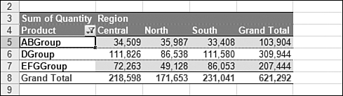
You need to add additional definitions for DGroup and EFGGroup. When you finish, these items are added to the end of the product list. The calculations work. As shown in Figure 12.34, the 103,904 reported for the ABGroup total is really the result of adding 50,616 and 53,288. However, the grand total shown in Row 19 has increased from 621,292 to 1,242,584. It is very easy to report the wrong numbers when you use calculated items.

Figure 12.34. Using calculated items causes the grand total in Row 19 to be wrong.

The only way that grouping items would make sense is if you used the Product filter to hide all the detail items and show only the calculated items, as shown in Figure 12.35.

Figure 12.35. Using calculated items makes sense only if you hide the items that make up the calculated items or remove the grand totals.

Instead of using calculated items, you should consider using the grouping functionality, as discussed in the following section.

Organizing a Hierarchy by Using Grouping

As shown in the previous section, using Calculated Items can lead to wrong results in the pivot table totals. You should consider defining subtotals along a dimension by using the Grouping feature instead.

For effective grouping, you will select item labels that make up a group and then click on the Group Selection icon.

For example, consider the pivot table shown in Figure 12.32. Select the products that make up the first group (that is, Cells A5:A6). On the Options ribbon, you click the Group Selection icon to group these products into a group. As shown in Figure 12.36, after you group the first items, a new Column A is added, called Product2. The first items are grouped into a new value called Group1. All the other items are in their own groups. This is okay; you can fix it with a few more clicks.

Figure 12.36. After you group the first few items, the remaining items fall into their own individual groups.

To build the D group, you select Cells B7 through B11. Then you click Group Selection to form a group of these items. Next, you select cells B12:B16 and click Group Selection to make the final group. The pivot table now has a completely new field, which you can easily expand or collapse, as shown in Figure 12.37.

Figure 12.37. You group the remaining items.

At this point, you have defined groups along a dimension. Excel shows the items in their various groups, but there are no totals for each group. To add subtotals to the analysis, follow these steps:

1. From the Styles ribbon choose Subtotals and then Show Subtotals.
2. Select Field Settings and give the grouped field a meaningful name. In the current example, something like Product Line would be appropriate.
3. At this point, the various groups will have generic names like Group1, Group2, etc. Select a cell with a group name. Right in the cell, type the new name AB Group.
4. Select the remaining group name cells and rename them.

The final report is shown in Figure 12.38.

Figure 12.38. Using the group selection and a few modifications, you can add a new dimension for the product line managers.

Showing Percentages Instead of Values

Figure 12.39 shows a report of profit by product and region. This report shows revenue in what is known as Normal view. Excel provides many additional views that can show any value field as a percentage of a total.

Figure 12.39. The Normal view of profit shows actual dollars in each cell.

To select a different view, you first select any value cell and then choose Field Settings from the Active Field group of the Options ribbon.

The Data Field Settings dialog appears. Its Show Data As tab stores all the percentage options. You can select any of the following options from the Show Data As tab without specifying additional information:

• Normal—Shows actual numbers.
• % of Row—Calculates the percentage of the row.
• % of Column—Calculates the percentage of the column.
• % of Total—Calculates the percentage of the grand total.
• Index—Assigns a relative importance of each cell in the pivot table.

The following option from the Show Data As tab requires that you specify a base field:

• Running Total In—Calculates a cumulative total as you go down the column.

The other three options on the Show Data As tab allow you to choose a base field and a base item:

• Difference From—Calculates a change from a base item.
• % Of—Calculates a percentage of a base item.
• % Difference From—Calculates a percentage difference from a base item.

Figure 12.40 shows a report that displays revenue as the percentage of the row. Each row adds up to a grand total of 100%. This type of report is useful for spotting trends by region. For example, you can see in Figure 12.40 that for some reason, Product D776 does much better in the central than most other products.

Figure 12.40. You can use this report to see how each product does by region.

Figure 12.41 shows revenue as a percentage of the column. Each column adds up to 100%. This is useful for comparing products within a region. You can see in this figure that Product D850 is the most important product in the north, whereas F495 seems to be a major component of southern sales.

Figure 12.41. You can use this report to see which products are important in each region.

The final percentage option is to take a percentage of the total. In this case, each cell in B5:E15 would represent a percentage of the grand total in E16.

Calculating the Difference from One Day to Another Using the Difference From Fields

The last type of setting for Show Data As are the Difference settings. These settings are the most complex. They allow you to compare all of the values along a dimension to another value along the same dimension.

The settings can be absolute, where every day’s sales is compared to the sales on the first day of the dataset. Or, the settings can be relative, where every day’s sales are compared to the previous day.

These final settings—the difference settings—round out a diverse group of powerful Show Data As options. The options provide nearly unlimited flexibility.

Consider the report in Figure 12.42. Each column from B through F shows off a different type of Show Data As setting. Column B shows the data as normal. Column C shows a running total. Column D shows a percentage of total. Column E uses the tricky Difference from Yesterday. Column F uses the difference from the first day in the period.

Figure 12.42. This report shows five views of revenue.

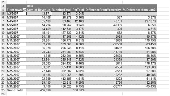
This section walks you through how to set up the report shown in Figure 12.42. In this report, each column shows a different view of revenue for January 2007.

If you wished to build a report similar to the one in Figure 12.42, you actually have to drag the same field to the Σ Values section several times. Each copy of the value field will have a different setting in the Show Data As area.

The following steps illustrate how each of the five columns in Figure 12.42 were defined:

1. Build a pivot table with Date in the Row Labels section and Revenue in the Σ Values section.
2. Filter the dates to include values in January 2007.
3. Drag the Revenue field to the Σ Values section four additional times.
4. Select Cell C5 (the first cell in the Revenue2 field) and then click Data Field Settings. Change the field name to RunningTotal. In the Show Data As drop-down, select Running Total In and then specify that you want to see the running total in the Date field. Finally, choose Date as the base field, as shown in Figure 12.43.

   Figure 12.43. A running total requires you to specify a base field.

   

5. Select Cell D5 (the first cell in the Revenue3 field) and then click Data Field Settings. Name the field PctTotal. Click the Show Values As tab. In the dropdown for Show Values As, choose “% of column”.
6. Select Cell E5 (the Revenue4 field) and then click Data Field Settings. Change Custom Name to DifferenceFromYesterday and set the Show Data As value to Difference From. Specify both a base field and a base item. The base field is the date item. For the Base item, choose (Previous), as shown in Figure 12.44, to compare each day’s sales to the previous day’s sales.

   Figure 12.44. Each of the Difference From settings requires a base field and a base item.

   

7. Select Cell F5 (the Revenue5 field) and then click Data Field Settings. In this case, choose % Difference From. The base field is still the Date field, but you want the base item to be the first day of the month, so choose 1/2/2007, as shown in Figure 12.45. Each value in this column then compares the day’s sales to the sales on the first day of the month.

Figure 12.45. In this case, each cell compares the current day’s sales to the sales on a specific day.

Figure 12.46. You need to redefine many of the Difference Of calculations after pivoting a table.

Exploring Interesting Uses for Pivot Tables

So far in this chapter, you have used pivot tables to perform various summary analyses, which is the reason pivot tables were invented. However, pivot tables are so easy to create and use that they often provide the quickest way to accomplish a task. The following sections describe some other uses for pivot tables.

Generting a Unique List

One quirky use of pivot tables is to generate a unique list of values in any field. For example, say you have a dataset that has 1,126 rows of transactional data. You need to quickly produce a unique list of the customers in the dataset. Although you could click the new Remove Duplicates icon on the Data ribbon to destructively find the unique customers, you can instead use a pivot table to do this in three clicks of the mouse:

1. Select a cell in your dataset and click the PivotTable icon on the Insert ribbon.
2. Click OK to accept the defaults on the Create PivotTable dialog.
3. Select Customer in the PivotTable Field List box.

You end up with a unique list of customers, as shown in Figure 12.47. You can copy this list and use Paste Special Values to move the list wherever you might need it to be.

Figure 12.47. Using pivot tables has always been the fastest way to get a unique list, and it is even faster in Excel 2007.

Counting Records

Another unusual use for pivot tables is to count how many records meet certain criteria. These datasets may contain columns of text without a single number anywhere in the range. You can still use a pivot table to analyze the data.

For example, Figure 12.48 shows a dataset that has no numeric data at all. It is a log of all the quality errors on a manufacturing line. Even though there is nothing to add up, you can analyze this data by using a pivot table. Follow these steps:

Figure 12.48. This dataset has no numeric data, but will be great in a pivot table.

1. Choose Insert, PivotTable and accept the default location.
2. Choose the Defect field to see a unique list of defects. Then drag the Defect field to the Σ Values section of the table. Because the field contains text, Excel automatically chooses to count the field instead of sum it.
3. Move the Line field to the Column Labels section of the table.

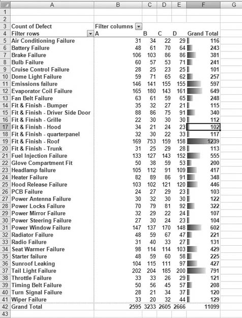
Figure 12.49 shows the completed pivot table with a data bar added to the grand total. It looks like the biggest problem is in Fit & Finish – Roof.

Figure 12.49. By counting the defects, you see that there is a problem in the Roof department.

Once you have produced one view of your data with a pivot table, you can use the flexibility of a pivot table to further analyze the data.

In the previous example, the pivot table indicated that there might be a problem with one particular step of a manufacturing process. However, there are additional fields in the underlying dataset that are not part of the analysis.

If you use the Report Filter to limit the report to just data for the one problematic manufacturing step, you can add additional fields to the pivot table to analyze if the problem started on a certain date, or is limited to a certain line or a certain shift.

To further analyze the table, follow these steps:

1. Move Defect from Row Labels to Report Filter and select the Roof item.
2. Move the Date field to the Row Labels section, as shown in Figure 12.50.

Figure 12.50. Pivot a few more fields, and you have a picture that the problem started on the B line toward the end of the month.

In the finished pivot table, shown in Figure 12.50, you can see that something happened on the 28th of the month that started causing a problem on the B line. By the 30th of the month, the problem had spread to the A, C, and D lines. You can guess that some new shipment of defective material probably arrived in the plant around this time frame.

This is just one example of the analysis that can be done by filtering a pivot table. The initial pivot table identified that the problem was in one area of the plant. Subsequent versions of the pivot table focused on that one area and brought more data to the table to locate the source of the problem.

Comparing Two Lists

One common hurdle in Excel is comparing data in two lists. You might have a snapshot of data from last week or last month and a new snapshot from today. How can you figure out what changed from the first list to the second list?

In the real world, some items from the first list will be deleted. Some items in the first list will get new values. Some items will appear on the second list that were never on the first list.

Most people attack this problem manually, comparing the two printed lists with a highlighter, trying to find the items that stayed the same and finding the items that changed.

A clever way to compare the lists is to use a pivot table. The data from both lists is copied into a new consolidated list. The records from each list are identified as being from either the original or latest list.

When you create a pivot table with the item key as the Row Label, the identifier as the column label, and the values, you can quickly see which items changed from list to list.

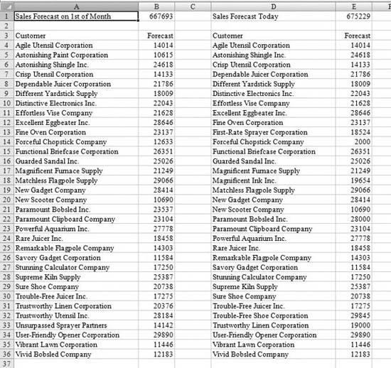
Specifically, say that you have two lists. List 1 is the sales forecast from last week. List 2 is the sales forecast from today. Both lists happen to have 33 records, but they are not the same 33 records!

Some customers are new, some were deleted, and some were changed. How can you quickly find out what changed between the two forecasts? To figure it out, follow these steps:

Figure 12.51. What changed between forecasts?

1. Add a new field called WhichForecast. In this field, use the value First for all the original forecasts.
2. Copy the new forecast beneath the original forecast and add the value Now for the new field.
3. Create a pivot table with Customer in the Row Labels section, WhichForecast in the Column Labels section, and Forecast in the Σ Value area.
4. Select the First header. Then select Options, Tools, Pivot Formulas, Insert Calculated Item to define the calculation Change = Now – First.

The result is the pivot table shown in Figure 12.52. In this view, you can quickly see that the forecasts for Astonishing Paint, Trustworthy Utensil, and Unsurpassed Sprayer were lost in the past week. New forecasts for First-Rate Sprayer, Magnificent Ink, and Trouble-Free Shoe appeared. Forceful Chopstick and Paramount Bobsled recorded minor changes.

Figure 12.52. You combine the two lists into a single list with a new field and then generate a pivot table to compare.

Figure 12.53. When you use the mouse to build a formula that contains cells in a pivot table, Excel substitutes GetPivotData functions for the cell address.

Grouping by Week

A previous example showed how to group daily dates up to months, quarters, or years. Occassionally, someone will have a need to group daily dates up to weeks. Even though the Grouping dialog doesn’t offer grouping by week, you can achieve this effect by doing the following:

1. Select a date field and click the Group Field icon on the Options ribbon.
2. In the Grouping dialog, choose to group only by days. This enables the Number of Days spin button in the lower-right corner.
3. Dial the Number of Days spin button up to 7 days. Because this dataset starts on January 2, 2007 (a Tuesday), your default weeks would run Tuesday through Monday.
4. If you want your weeks to run Monday through Sunday, change the Starting At value to 1/1/2007. If you want your weeks to run Sunday through Saturday, change the Starting At value to 12/31/2006.

Figure 12.54 shows the Grouping dialog box and the result of following these steps.

Figure 12.54. Even though weeks are not an option, you can group by them by using the Number of Days option.

Finding More Information on Pivot Tables

A number of aspects of pivot tables are not covered in this and the previous two chapters. Other parts of this book provide further information on pivot tables:

• If you want to know how to create a pivot table from Access data, see see Chapter 37, “Interacting with Other Office Applications.”
• If you want to know how to create pivot charts from pivot tables, see Chapter 15, “Charting.”
• Pivot table source data can automatically expand if your data is set up as a table. For information on using tables in Excel 2007, see Chapter 8, “Fabulous Table Intelligence.”