
Chapter 23. Using Everyday Functions: Math, Date and Time, and Text Functions
In this chapter
Examples of Math Functions 458
Examples of Date and Time Functions 490
Examples of Text Functions 505
Excel offers many functions for dealing with basic math, dates and times, and text. This chapter describes the functions found under the Date & Time icon and the Math & Trig icon on the Formulas ribbon.
Table 23.1 provides an alphabetical list of all of Excel 2007’s math functions. Detailed examples of these functions are provided later in this chapter.
Table 23.1. Alphabetical List of Math Functions


Table 23.2 provides an alphabetical list of all of Excel 2007’s date and time functions. Detailed examples of these functions are provided later in this chapter.
Table 23.2. Alphabetical List of Date and Time Functions


Table 23.3 provides an alphabetical list of all of Excel 2007’s text functions. Detailed examples of these functions are provided later in this chapter.
Table 23.3. Alphabetical List of Text Functions


Examples of Math Functions
The most common formula in Excel is a formula to add a column of numbers. In addition to SUM, Excel offers a wide variety of mathematical functions.
Using SUM to Add Numbers
The SUM function is by far the most commonly used function in Excel. This function can add numbers from one or more ranges of data.
Syntax: =SUM(number1,number2,...)
The SUM function adds all the numbers in a range of cells. The arguments number1,number2,... are 1 to 255 arguments for which you want the total value or sum.
A typical use of this function is =SUM(B4:B12). It is also possible to use =SUM(1,2,3). In the latter example, you cannot specify more than 255 individual values. In the former example, you can specify up to 255 ranges, each of which can include thousands of cells.
In Figure 23.1, cell B25 contains a formula to sum three individual cells: =SUM(B17,B19,B23).
Figure 23.1. A variety of SUM formulas

It is unlikely that you will need more than 255 arguments in this function, but if you do, you can group arguments in parentheses. For example, =SUM((A10,A12),(A14,16)) would count as only 2 of the 255 allowed arguments.
If a text value that looks like a number is included in a range, the text value is not included in the result of the sum. Strangely enough, if you specify the text value directly as an argument in the function, Excel does add it to the result. For example, =SUM(1,2,"3") will be 6, yet =SUM(D4:D6) in Figure 23.1 will result in 3.
If one cell in a referenced range contains an error, the result of the SUM function is an error.
It is valid to create a spearing formula. This type of formula adds the identical cell from many worksheets. For example, =SUM(Jan:Dec!B20) would add Cell B20 on all 12 sheets between January and December.
To quickly enter a SUM formula, you can press Alt+= or click the AutoSum icon on the Formulas ribbon. In Figure 23.2, pressing the AutoSum icon will add totals to the 13 selected blank cells all at once (see Figure 23.3).
Figure 23.2. The AutoSum icon (the Greek letter sigma) adds sum formulas to all the selected cells at once.

Figure 23.3. After clicking AutoSum, the total formulas are automatically entered.

Using COUNT or COUNTA to Count Numbers or Nonblank Cells
A number of functions process nonblank cells. =COUNT counts all the numeric or date cells in a range. =COUNTA counts all the nonblank cells in a range.
Caution
COUNT and COUNTA are found in the Statistical drop-down under the More Functions icon of the Formulas ribbon.
Syntax: =COUNT(value1,value2,...)
The COUNT function counts the number of cells that contain numbers and also numbers within the list of arguments. You use COUNT to get the number of numeric entries in a range or array.
The arguments value1, value2,... are 1 to 255 arguments that can contain or refer to a variety of different types of data, but only numbers are counted.
Note that while a single error cell in a range causes the SUM function to return an error, the same condition is ignored in the COUNT function.
=COUNT(1,2,"3") results in the text entry being counted. If you refer to a range that contains text that looks like a number, the text is not included in the count.
Syntax: =COUNTA(value1,value2,...)
COUNTA counts the number of cells that are not empty and the values within the list of arguments. You use COUNTA to count the number of cells that contain data in a range or an array.
The arguments value1, value2,... are 1 to 255 arguments representing the values you want to count. In this case, a value is any type of information, including empty text ("") but not including empty cells. If an argument is an array or a reference, empty cells within the array or reference are ignored. If you do not need to count logical values, text, or error values, you should use the COUNT function.
Note that error cells are included in the results from COUNTA.
Choosing Between COUNT and COUNTA
The key to choosing between COUNT and COUNTA is to analyze the data that you want to count. In Figure 23.4, someone has used X’s in Column B to indicate that training has been started. In this case, you would use COUNTA to get an accurate count. Column C contains dates (which are treated as numeric). In Column C, either COUNT or COUNTA returns the correct result. Column D has a mix of text and numeric entries. If you want to count how many people took the test, you use COUNTA. If you want to count how many people received a numeric score, you use COUNT.
Figure 23.4. Whether you use COUNT or COUNTA depends on whether your data is numeric. COUNT counts only dates and numeric entries. COUNTA counts anything that is nonblank.

Caution
Using more than 30 arguments in COUNT or COUNTA causes backward compatibility problems with Excel 2003 and earlier.
Using ROUND, ROUNDDOWN, ROUNDUP, INT, TRUNC, FLOOR, CEILING, EVEN, ODD, or MROUND to Remove Decimals or Round Numbers
A wide variety of functions—including ROUND, ROUNDDOWN, ROUNDUP, INT, TRUNC, FLOOR, CEILING, EVEN, ODD, and MROUND—can be used to round a result or to remove decimals from a result.
Syntax: =TRUNC(number), =INT(number), =EVEN(number), and =ODD(number)
The TRUNC, INT, EVEN, and ODD functions always change a number to an integer. The syntax in each case is similar: The function accepts a single number or a single cell containing a number.
To remove the decimals from a result, you use the =TRUNC function. This truncates a number to the integer portion of the number. For example, =TRUNC(1.9) is 1, and =TRUNC(-1.9) is -1.
To remove the decimals from a result and always round down to the next lowest integer, you use =INT. For positive numbers, TRUNC and INT return identical values. There is a subtle difference between TRUNC and INT. When you have a negative number, INT rounds away from zero to produce the next lowest integer. Thus, =INT(-1.1) is -2.
EVEN rounds a number away from zero to the next even integer. For example, =EVEN(3) is 4, and =EVEN(-3) is -4. If the number is already an even integer, no adjustment is made; for example, =EVEN(6) is 6. This function is ideal for ordering products packed two to a case.
ODD rounds a number away from zero to the next odd integer. For example, =ODD(1.1) is 3, and =ODD(-3.1) is -5. If the number is already an odd integer, no adjustment is made.
Figure 23.5 compares the results of TRUNC, INT, EVEN, and ODD.
Figure 23.5. TRUNC and INT are nearly identical, except when the numbers become negative.

Syntax: =ROUND(number,num_digits), ROUNDUP(number,num_digits), and ROUNDDOWN(number,num_digits)
Three more functions—ROUND, ROUNDUP, and ROUNDDOWN—round a number to a specified number of decimal places. They all take the following arguments:
number—This is the number you want to round.num_digits—This specifies the number of digits to which you want to roundnumber.
With ROUND, if the number of digits is zero, the number is rounded to the nearest integer, following these rules:
- Values up to 0.49 are rounded toward zero. For example,
ROUND(1.49,0)results in1, andROUND(-1.49,0)results in-1. - Values of 0.5 and above are rounded away from zero. For example,
ROUND(1.5,0)results in2, andROUND(-1.5,0)results in-2.
If the num_digits is positive, the number is rounded to have the specified number of decimal places. If the number of digits is negative, the number is rounded to the left of the decimal point. For example, ROUND(117,-1) is rounded to the nearest 10, or a value of 120.
To override the rounding rules, you can use ROUNDDOWN or ROUNDUP:
- The
ROUNDDOWNfunction always rounds toward zero. For example,=ROUNDDOWN(1.999,0)rounds to1, and=ROUNDDOWN(-19.999,0)rounds to-19. You might use this function when judging a contest in which if the entrant does not completely finish a task, he or she does not get credit for the unfinished portion of the task. - The result of the
ROUNDUPfunction always rounds away from zero. For example,=ROUNDUP(1.01,0)rounds up to2, and=ROUNDUP(-1.01,0)rounds to-2. You might use this function when calculating prices because if the customer uses any fractional portion of a product, he or she is charged for the complete product.
Using a negative number for the number of digits provides an interesting result. If you need to round a number to the nearest thousand, you can indicate that it should be rounded to -3 decimal places. For example, ROUND(1,234,567,-3) would be 1,235,000.
Figure 23.6 compares ROUND, ROUNDUP, and ROUNDDOWN.
Figure 23.6. These three functions always round to a power of 10.

Syntax: =MROUND(number,multiple), =CEILING(number,signifigance), and =FLOOR(number,significance)
The last three functions in this group—MROUND, CEILING, and FLOOR—round a number to a certain multiple. They require you to enter the number and the multiple to which to round. They all take the following arguments:
number—This is the number you want to round.multipleorsignificance—This is the nearest multiple that you want to round toward. Note that ifnumberis negative,multipleorsignificancemust also be negative.
Say that you handle pricing for a line of products. Your general rule is to mark up the product cost, which results in a series of strange prices, such as $185.9375, as shown in Figure 23.7. To round each price to the nearest increment of $5, you would use =MROUND(C2,5). You could also use MROUND to round to the nearest quarter: =MROUND(C2,0.25).
Figure 23.7. MROUND rounds a price to a certain multiple. Here, Column D is the calculated prices rounded to the nearest $5.

The multiple argument in MROUND is allowed to be negative.
There is one strange behavior to look out for with MROUND, FLOOR, and CEILING. If the number is negative, you must ensure that the second argument for the function is also negative. There certainly could be situations in which you don’t know in advance whether your numbers will be negative. If you think that your numbers might be a mix of positive and negative values, you should use =MROUND(C2,5*SIGN(C2)). This will ensure that the second parameter matches the sign of the first parameter.
In other situations, you may want to round a number up to a certain multiple. Figure 23.8 shows a requisition list. Column A shows the quantity needed, and Column B shows the item. The purchasing agent discovered a vendor who offers a significant discount, but only if you buy in complete case quantities. Column C shows the size of the case for each product. To calculate the total number to order, you need to round a number in Column A up to the nearest multiple of the case size found in Column C. You use =CEILING(A4,C4) to achieve this effect.
Figure 23.8. CEILING rounds a number up to the next multiple.

CEILING rounds away from zero. If you use =CEILING(-9,-6), the function rounds -9 to -12.
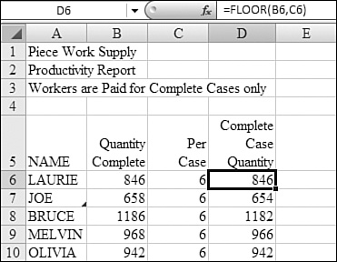
The FLOOR function rounds a number to the next lowest multiple. Say that you employ several student workers who do piece work. They assemble products and then pack them six to a case. Your contract with the workers says that you only pay for complete cases. Column B in Figure 23.9 shows the total number of units assembled. You use =FLOOR(B6,6) to round this quantity down to the nearest multiple of six. Note that if the value is already a multiple of six, as in Cell B10, FLOOR does not change the number.
Figure 23.9. FLOOR rounds a number down to the next multiple.
All the functions for rounding can actually be replaced with a clever combination of INT and ROUND functions. If you receive a spreadsheet from an old-time Lotus 1-2-3 user, you may see formulas like the ones in Figure 23.10:
- Cell B13 is equivalent to using
MROUNDwith a multiple of 20. The formula divides 135 by 20, giving 6.75.ROUNDrounds this to 7. Finally, outside the parentheses, the formula multiplies by 20 to arrive at the answer of 140. - Cell C13 is equivalent to using
FLOORwith a significance of 20. The formula divides 135 by 20, giving 6.75. TheINTremoves the decimal places, leaving the integer 6. The formula then multiplies this result by 20 to arrive at 120. - Cell D13 is equivalent to using
CEILINGwith a significance of 20. The formula divides 135 by 20, giving 6.75. Next, the formula adds just less than 0.5 to make sure that any value greater than 6 is rounded up to 7. Finally, the result is multiplied by 20 to arrive at 140.
Figure 23.10. A combination of ROUND and INT can replace any of the eight other functions used for rounding.

In previous versions of Excel, functions such as MROUND were not part of the core Excel. They were enabled when someone installed the Analysis Toolpack. Because new Excel users might never have installed the Analysis Toolpack, some people would avoid using MROUND and would instead write the formulas as shown in Figure 23.10. Now that Microsoft has elevated all the Analysis Toolpack functions to be part of the core Excel 2007 product, it is safe to use those functions.
Using SUBTOTAL Instead of SUM with Multiple Levels of Totals
Consider the dataset shown in Figure 23.11. This report shows a list of invoices for each customer. Someone has manually inserted rows and used the SUM function to total each customer. Cells C5, C10, C15, and so on contain a SUM function.
Figure 23.11. Whoever manually summed these rows doesn’t know about the Subtotal command on the Data ribbon.

It would be very difficult to enter a grand total at the bottom of this dataset. You might have to enter a long formula that only points at the summary rows. In this particular case, the formula to provide a grand total for 15 customers would be possible, as shown in Figure 23.12. If you had 500 customers, however, the formula would be nearly impossible to enter.
Figure 23.12. It is difficult to enter the grand total formula.
Many accountants can teach you the old accounting trick that you can actually total the entire column and divide by two in order to get the grand total. This is based on the assumption that every dollar is in the column twice: once on the detail row and once on the summary row. As shown in Figure 23.13, this trick does work, but it is hard to explain to your manager why it works.
Figure 23.13. The old accounting trick of adding an entire column and dividing by two works but is hard to explain.

The solution is to use the SUBTOTAL function. This powerful function is relatively new; it was introduced in Excel 97.
Tip From
![]()
The best way to insert the SUBTOTAL function is to use the Subtotals icon on the Data ribbon, as described in Chapter 35, “More Tips and Tricks for Excel 2007.” However, you can set up these functions manually.
Syntax: =SUBTOTAL(function_num,ref1,ref2,...)
In its default use, SUBTOTAL works just like the SUM function, except it throws out other instances of the SUBTOTAL function within the range being summed. The SUBTOTAL function takes the following arguments:
function_num—This is a number from1to11. The most common function number is the number9, which (for no logical reason) is used to sum. When Microsoft introduced theSUBTOTALfunction, it offered 11 options:AVERAGE,COUNT,COUNTA,MAX,MIN,PRODUCT,STDEV,STDEVP,SUM,VAR, andVARP. It just happens thatSUMis the ninth item in this list when these functions are arranged alphabetically in the English language, so9became the function number forSUM.ref1,ref2,...—These are up to 29 ranges or references that you want to subtotal. Unlike withSUM, the references in aSUBTOTALfunction cannot be 3D references.
Any other nested subtotals in the range are ignored to prevent double counting.
The SUBTOTAL function always ignores rows hidden as the result of a filter. This makes the SUBTOTAL function great in combination with autofilter, as you’ll see later in this chapter, in Figure 23.15.
A feature added in Excel 2002 is that you can add 100 to the function number in order to prevent Excel from including rows hidden by using the Hide command. Note that this functionality works only with hidden rows. If you hide columns and attempt to subtotal in a horizontal fashion, the hidden columns are not ignored.
Table 23.4. Function Arguments for SUBTOTAL

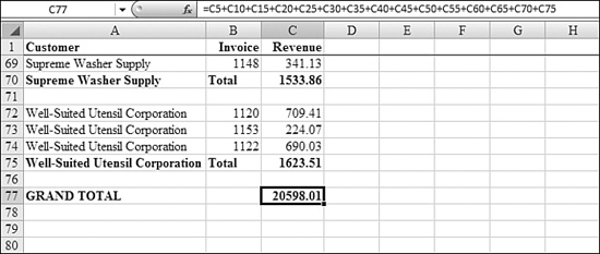
In Figure 23.14, the customer summary rows were built with the SUBTOTAL function, allowing the grand total row to be calculated with the simple formula =SUBTOTAL(9,C2:C76).
Figure 23.14. When you use SUBTOTAL instead of SUM for the customer totals, the problem of creating a grand total becomes simple.

Using SUBTOTAL Instead of SUM to Ignore Rows Hidden by a Filter
If you are using autofilter to query a dataset, you can use the SUBTOTAL function instead of the SUM function in order to show the total of the visible rows. In Figure 23.15, Cell E1 contains a SUM function, which totals rows whether they are visible or not. Cell E2 contains a SUBTOTAL function. As you use the autofilter drop-downs to show just rows for sales of J730 by Jamie, the SUBTOTAL function updates to reflect the total of the visible rows. This makes the SUBTOTAL function a great tool for ad hoc reporting.
Figure 23.15. The SUBTOTAL function in Cell E2 ignores rows hidden as the result of a filter.

Note
Although the function in Figure 23.15 uses the function number 109, the Subtotal command always ignores rows hidden as the result of a filter. =SUBTOTAL(9,E5:E5090) would return an identical result.
Using RAND and RANDBETWEEN to Generate Random Numbers and Data
There are a number of situations in which you might want to generate random numbers. Excel offers two functions to assist with this process: RAND and RANDBETWEEN.
Syntax: =RAND()
The RAND function returns an evenly distributed random number greater than or equal to 0 and less than 1. A new random number is returned every time the worksheet is calculated.
=RAND() generates a random decimal between 0 and 0.99999. Whether you are a teacher trying to randomly assign the order for book report presentations, or the commissioner of a fantasy football league trying to figure out the draft sequence, =RAND() can help.
If you want to use RAND to generate a random number but don’t want the numbers to change every time the cell is calculated, you can enter =RAND() in the formula bar and then press F9 to change the formula to a random number.
To generate a random number greater than or equal to 0 but less than 100, you can use RAND()*100.
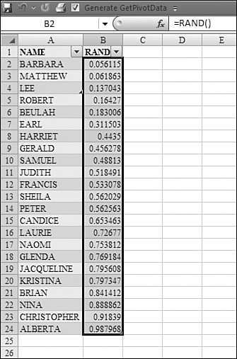
To generate a random sequence for a list, you select a blank column next to your data and enter =RAND() in the column. Every time you press the F9 key, the column generates a new set of random numbers. You might want to agree up front with the draft participants that you will press F9 three times to randomize the list and then convert the formulas to values. To do so, you follow these steps:
- Enter the heading
Randomin Row 1 next to your data. - Enter
=RAND()in Cell B2. - Move the cell pointer to Cell B2 and double-click the fill handle.
- Turn off automatic calculation. From the Office icon in the upper-left corner, choose Excel Options, Formulas and then choose Manually in the Calculation options section. Click OK to return to the worksheet.
- Press the F9 key three times.
- Choose one cell in Column B.
- From the Home ribbon, choose Sort & Filter, Sort Smallest to Largest. The new sequence of items in Column A is a random sequence (see Figure 23.16).
Figure 23.16. Barbara gets to draft first in this season’s fantasy football league, thanks to the RAND function.
You can also use this technique to select a random subset from a dataset. If your manager wants you to contact every 20th customer, you can select all the customers where =RAND() is 0.05 or less.
Syntax: =RANDBETWEEN(bottom,top)
Whereas =RAND() returns a random decimal, =RANDBETWEEN generates an integer between two integers.
The RANDBETWEEN function returns a random number between the numbers you specify. A new random number is returned every time the worksheet is calculated. This function takes the following arguments:
bottom—This is the smallest integerRANDBETWEENcan return.top—This is the largest integerRANDBETWEENcan return.
To generate random numbers between 50 and 59, inclusive, you use =RANDBETWEEN(50,59). RANDBETWEEN is easier to use than =RAND to achieve random integers; with =RAND, you would have to use =INT(RAND()*10)+50 to generate this same range of data.
Even though RANDBETWEEN generates integers, you can use it to generate sales prices or even letters. =RANDBETWEEN(5000,9900)/100 generates random prices between $50.00 and $99.00.
The capital letter A is also known as character 65 in the ASCII character set. B is 66, C is 67, and so on up through Z, which is character 90. You can use =CHAR(RANDBETWEEN(65,90)) to generate random capital letters.
Many of the product SKUs in this book were generated using =CHAR(RANDBETWEEN(65,90))& RANDBETWEEN(101,199).
Figure 23.17. RANDBETWEEN can generate integers, or, with a little creativity, prices or letters.

Choosing a Random Item from a List
In Figure 23.18, you want to randomly assign employees to certain projects. The list of projects is in Column A. The list of employees is in E2:E6. As shown in Figure 23.18, the function for B2:B11 is =INDEX($E$2:$E$6,RANDBETWEEN(1,5)).
Figure 23.18. I wonder if Dilbert’s pointy-haired boss assigns projects this way.

Using =ROMAN() to Finish Movie Credits
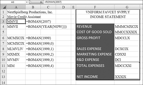
Excel can convert numbers to Roman numerals. If you stay in the theater after a movie until the very end of movie credits, you will see that the copyright date is always expressed in Roman numerals. If you are the next Steven Spielberg, you can use =ROMAN(2007) or =ROMAN(YEAR(Now())) to generate such a numeral.
Caution
In a previous book, I joked that if you had bad financial news to share with stockholders, you might try converting your financial statement to Roman numerals. However, you can use the ROMAN function only in limited circumstances. Negative numbers, 0, and numbers over 3,999 cannot be represented with the ROMAN function.
Syntax: =ROMAN(number,form)
The ROMAN function converts an Arabic numeral to Roman, as text. This function takes the following arguments:
number—This is the Arabic numeral you want converted.form—This is a number that specifies the type of Roman numeral you want. The Roman numeral style ranges from Classic to Simplified, becoming more concise as the value offormincreases.
There are some arcane rules with Roman numerals. In classic Roman numbers, an I before a V is used to indicate the number 4. In classic Roman numbers, it is valid to use an I before a V or an X, but it is not valid to use an I before an L, a C, a D, or an M.
As shown in Figure 23.19, the form argument allows Excel to bend these rules progressively more:
ROMAN(1999,0)results inMCMXCIX. TheMis 1000, theCMis 900, theXCis 90, and theIXis 9; 1000 + 900 + 90 + 9 = 1999ROMAN(1999,1)results inMLMVLIV. TheMis 1000, theLMis 950, theVLis 45, and theIVis 4; 1000 + 950 + 45 + 4 = 1999.ROMAN(1999,2)results inMXMIX. TheMis 1000, theXMis 990, and theIXis 9; 1000 + 990 + 9 = 1999.ROMAN(1999,3)results inMVMIV. TheMis 1000, theVMis 995, and theIVis 4; 1000 + 995 + 4 = 1999.ROMAN(1999,4)results inMIM. TheMis 1000 and theIMis 999; 1000+999 = 1999.
Figure 23.19. You can create movie credit dates with Cell A3 or present bad news with F1:G13. Compare the various forms of Roman numerals in A7:A11.
Using ABS() to Figure Out the Magnitude of ERROR
Say that you work for a local TV station, and you want to prove that your forecaster is more accurate than those at the other stations in town. The forecaster at the rival station in town is horrible—some days he misses high, and other days he misses low. The rival station uses Figure 23.20 to say that his average forecast is 99% accurate. All those negative and positive errors cancel each other out in the average.
Figure 23.20. ABS measures the size of an error, ignoring the sign.

The ABS function measures the size of the error. Positive errors are reported as positive, and negative errors are reported as positive as well. You can use =ABS(A2-B2) to demonstrate that the other station’s forecaster is off by 20 degrees on average.
Syntax: =ABS(number)
The ABS function returns the absolute value of a number—that is, the number without its sign. With this function, the argument number is the real number of which you want the absolute number.
Using PI to Calculate Cake or Pizza Pricing
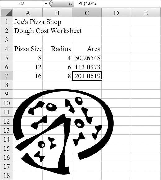
How many more ingredients are in a 16-inch pizza than an 8-inch pizza? Be careful—it is not double!
The formula for the area of a circle is π × r2. The radius of a circle is half the diameter. The function =PI() returns the constant for PI. You use =PI()*(B7/2)^2 to calculate the number of square inches in a 16-inch pizza. As shown in Figure 23.21, the 16-inch size contains nearly four times the area of an 8-inch circle.
Figure 23.21. Most pizza shops don’t have a dedicated cost accountant.
If your company makes anything round—drink coasters, drum heads, wedding cakes, pizzas, or Frisbees—you want to use =PI() when calculating your product cost.
Syntax: =PI()
The PI function returns the number 3.14159265358979, the mathematical constant π, accurate to 15 digits.
Using =COMBIN to Figure Out Lottery Probability
Your office lottery pool may agree to bet $1 on the lottery each week but to double the bet when the jackpot is a higher payout than the odds against winning.
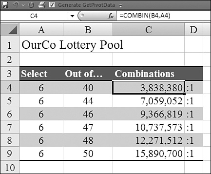
The COMBIN function can figure out the number of combinations for most lottery systems. If you have to correctly select 6 numbers out of a pool of 48 numbers, you can use =COMBIN(48,6) to find that there are 11.1 million combinations.
Figure 23.22 shows a variety of lottery odds.
Figure 23.22. The odds of winning the lottery in a 44-number games are twice as good as in a 50-number game.
Note
The COMBIN function assumes that you don’t care about the sequence of the numbers chosen. If you have to worry about the sequence, you should use =PERMUT, as described in Chapter 26, “Using Statistical Functions.”
Using FACT to Calculate the Permutation of a Number
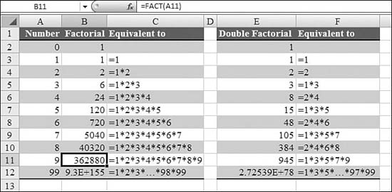
Let’s say that you have seven slides in a PowerPoint presentation. Furthermore, say you want to find the number of unique sequences in which the slides can be arranged; this is called the factorial of seven. You calculated this by using 7 × 6 × 5 × 4 × 3 × 2 × 1. To find the factorial of any positive integer, you use the FACT function.
Syntax: =FACT(number)
The FACT function returns the factorial of a number. The factorial of a number is equal to 1 × 2 × 3 × ... × number. number is the nonnegative number of which you want the factorial. If number is not an integer, it is truncated.
By definition, FACT(0) is 1.
There is a similar function called FACTDOUBLE. A double factorial multiplies every other number. For even numbers, this is a calculation such as
FACTDOUBLE(8) = 8*6*4*2. For odd numbers, the calculation is FACTDOUBLE(9) = 9*7*5*3*1.
Various factorials are shown in Figure 23.23.
Figure 23.23. Excel calculates the FACT and DOUBLEFACT of various numbers.
Note
It is difficult to find real-world uses for DOUBLEFACT. MathWorld.com notes some interesting uses for DOUBLEFACT(N) where N is less than zero, but Excel does not calculate DOUBLEFACT for negative numbers. Fans of the poker game Texas Hold’Em will be delighted to know that DOUBLEFACT is useful in calculating Texas Hold’Em probabilities. For complete details, look up Poker Probabilities (Texas Hold’Em) in Wikipedia.
Using GCD and LCM to Perform Seventh-Grade Math
My seventh-grade math teacher, Mr. Irwin, taught me about greatest common denominators and least common multiples. (For example, the least common multiple of 24 and 36 is 72. The greatest common denominator of 24 and 36 is 12.) I have to admit that I never saw these concepts again until my son Josh was in seventh grade. This must be permanently part of the seventh-grade curriculum.
If you are in seventh grade or you are assisting a seventh grader with his or her math lesson, you will be happy to know that Excel can calculate these values for you.
Syntax: =GCD(number1,number2,...)
The GCD function returns the greatest common divisor of two or more integers. The greatest common divisor is the largest integer that divides both number1 and number2 without a remainder.
The arguments number1, number2,... are 1 to 29 values. If any value is not an integer, it is truncated. If any argument is nonnumeric, GCD returns a #VALUE! error. If any argument is less than zero, GCD returns a #NUM! error. The number 1 divides any value evenly. A prime number has only itself and 1 as even divisors.
Syntax: =LCM(number1,number2,...)
The LCM function returns the least common multiple of integers. The least common multiple is the smallest positive integer that is a multiple of all integer arguments—number1, number2, and so on. You use LCM to add fractions with different denominators.
The arguments number1, number2,... are 1 to 29 values for which you want the least common multiple. If the value is not an integer, it is truncated. If any argument is nonnumeric, LCM returns a #VALUE! error. If any argument is less than one, LCM returns a #NUM! error.
Using MULTINOMIAL to Solve a Coin Problem
While the multinomial distribution is a fairly complex mathematical concept, the example below illustrates a fun puzzle that can be solved with the function.
Syntax: =MULTINOMIAL(number1,number2,...)
The MULTINOMIAL function returns the ratio of the factorial of a sum of values to the product of factorials. The arguments number1, number2,... are 1 to 29 values for which you want the multinomial. For example, MULTINOMIAL(a,b,c,d) is (a+b+c+d)! / a!b!c!d!.
Say that you have a huge jar that contains hundreds of pennies, nickels, dimes, and quarters. You reach into the jar and pull out six coins. How many possible arrangements of the coins can there be? To picture this problem, you should sort the six types of coins from low to high. You can use three movable dividers to group the coins into denominations. In the left side of Figure 23.24, for example, you’ve arranged the dividers to indicate one penny, one nickel, three dimes, and one quarter. It is possible to pull out none of a particular coin. In the image on the right, you’ve pulled out five pennies and one dime. In this case, the dividers are adjacent for nickels and pennies. In every case, the quarter divider must always be at the bottom, so how many ways are there to arrange the other three dividers among six coins?
Figure 23.24. Solving this problem with MULTINOMIAL will amuse Boy Scout groups and middle school math students.

Someone figured out that the answer to this problem is the factorial of (Dividers + Coins) ÷ Factorial of Coins × Factorial of Dividers. In math terms, this is (3+6)! / 3!6!. Remarkably, Excel has a function for solving the coin problem. =MULTINOMIAL(3,6) performs the calculation (3+6)!/3!6!.
Using MOD to Find the Remainder Portion of a Division Problem
The MOD function is one of the obscure math functions that I find myself using quite frequently. Have you ever been in a group activity where everyone in the group was to count off by sixes? This is a great way to break up a group into six subgroups. It makes sure that friends who were sitting together get put into disparate groups.
Using the MOD function is a great way to perform this concept with records in a database. Perhaps for auditing, you need to check every eighth invoice. Or you need to break up a list of employees into four groups. You can solve these types of problems by using the MOD function.
Think way back to when you were first learning division. If you had to divide 43 by 4, you would have written that the answer was 10 with a remainder of 3. If you divide 40 by 4, the answer is 10 with a remainder of 0.
Note
MOD is short for modulo, the mathematical term for this operation. You would normally say that 17 modulo 3 is 2.
The MOD function divides one number by another and reports back just the remainder portion of the result. You end up with an even distribution of remainders. If you convert the formulas into values and sort, your data is broken into similar-size groups.
Syntax: =MOD(number,divisor)
The MOD function returns the remainder after number is divided by divisor. The result has the same sign as divisor. This function takes the following arguments:
number—This is the number for which you want to find the remainder.divisor—This is the number by which you want to divide number. Ifdivisoris0,MODreturns a#DIV/0!error.
The MOD function is good for classifying records that follow a certain order. For example, the SmartArt gallery contains 84 icons arranged with 4 icons per row. To find the column for the 38th icon, use =MOD(38,4).
The example in figure 23.25 assigns all employees to one of four groups.
Figure 23.25. To organize these employees into four groups, you use =MOD(ROW(),4). Then you paste the values and sort by the remainders.

Using QUOTIENT to Isolate the Integer Portion in a Division Problem
As you just learned, the MOD function isolates the remainder portion in a division problem. The QUOTIENT function isolates the integer portion in a division problem.
If you divide 43 by 4, the answer is 10 with a remainder of 3. The QUOTIENT function returns just the whole number 10 and ignores the remainder.
This function is great for calculating full cases of products. Say that you pay a worker for assembling products. You pay the worker each complete case of 4 items produced. If he produces 43 items in his shift, this is 10 complete cases. =QUOTIENT(43,4) would provide an answer of 10.
Syntax: =QUOTIENT(numerator,denominator)
The QUOTIENT function returns the integer portion in a division problem. You use this function when you want to discard the remainder in a division problem. This function takes the following arguments:
numerator—This is the dividend.denominator—This is the divisor.
If either argument is nonnumeric, QUOTIENT returns a #VALUE! error.
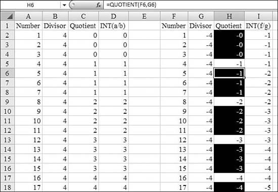
Many people simulate the QUOTIENT function by using the INT function. To keep the integer portion of a division, you could use =INT(43/4). However, QUOTIENT and INT differ when the result is negative. Whereas QUOTIENT(5,-4) returns -1, INT(5/-4) actually goes down to -2. Thus, using QUOTIENT is more accurate than using INT if the results might be negative. Figure 23.26 shows the differences between INT and QUOTIENT.
Figure 23.26. QUOTIENT is more accurate than INT when the result is negative.
Using PRODUCT to Multiply Numbers
The PRODUCT function multiplies a range of numbers by each other. Although you could calculate =PRODUCT(2,2), the PRODUCT function is designed to multiply all numbers in a range, such as =PRODUCT(A2:A50).
Syntax: =PRODUCT(number1,number2,...)
The PRODUCT function multiplies all the numbers given as arguments and returns the product. The arguments number1, number2,... are 1 to 30 numbers that you want to multiply. If you pass a single-cell argument that contains a text representation of a number, it is used in the multiplication. However, if one of the arguments is a multicell range, then any text entry in that range is ignored.
Using SQRT and POWER to Calculate Square Roots and Exponents
Most calculators offer a square root button, so it seems natural that Excel would offer a SQRT function to do the same thing. To square a number, you multiply the number by itself, ending up with a square. For example, 5 × 5 = 25.
A square root is a number that, when multiplied by itself, leads to a square. For example, the square root of 25 is 5, and the square root of 49 is 7. Some square roots are more difficult to calculate. The square root of 8 is a number between 2 and 3—somewhere close to 2.828. You can calculate the number with =SQRT(8).
A related function is the POWER function. If you want to write the shorthand for 6 × 6 × 6 × 6 × 6, you would say “six to the fifth power,” or 65. Excel can calculate this with =POWER(6,5).
Syntax: =SQRT(number)
The SQRT function returns a positive square root. The argument number is the number for which you want the square root. If number is negative, SQRT returns a #NUM! error.
Syntax: =POWER(number,power)
The POWER function returns the result of a number raised to a power. This function takes the following arguments:
number—This is the base number. It can be any real number.power—This is the exponent to which the base number is raised.
The POWER function works with all sorts of irrational numbers, such as 98.2 raised to the 3.4 power.
Figuring Out Other Roots and Powers
The SQRT function is provided because some math people expect it to be there. There are no equivalent functions to figure out other roots.
If you multiply 5 × 5 × 5 to get 125, then the third root of 125 is 5. The fourth root of 625 is 5. Even a $30 calculator offers a key to generate various roots beyond a square root. Excel does not offer a cube root function. In reality, even the POWER and the SQRT functions are not necessary. Chapter 20, “Understanding Formulas,” explains how the carat operator can be used to calculate powers and roots:
- =
6^3is 6 raised to the third power, which is 6 × 6 × 6, or 216 - =
2^8is 2 to the eighth power, which is 2 × 2 × 2 × 2 × 2 × 2 × 2 × 2, or 256
For roots, you can raise a number to a fractional power:
=256^(1/8)is the eighth root of 256. This is 2.=125^(1/3)is the third root of 125. This is 5.
Thus, instead of using =SQRT(25), you could just as easily use =25^(1/2). However, people reading your worksheets are more likely to understand =SQRT(25) than =25^(1/2).
Note
There is a specialized version of SQRT, SQRTPI, which is discussed in Chapter 27, “Using Trig, Matrix, and Engineering Functions.” This function first multiplies a number by PI and then takes the square root of the result. You can win a real pizza pie if you can think of a useful reason to do this. See Chapter 27.
Using SIGN to Determine the Sign of a Number
Although the SIGN function really belongs with the information functions, Microsoft groups it with the math functions. You can see it used in the MROUND function example shown previously in this chapter to prevent an error. Simply, =SIGN(number) reports whether number is negative, zero, or positive.
Syntax: =SIGN(number)
SIGN determines the sign of a number. It returns 1 if the number is positive, 0 if the number is 0, and -1 if the number is negative. The argument number is any real number.
Using COUNTIF and SUMIF to Conditionally Count or Sum Data
The COUNTIF and SUMIF functions are young and popular. As opposed to most functions that have been around since the 1980s, these functions were added in Excel 97. Math purists may point out that you could perform equivalent calculations by using DSUM or SUMPRODUCT or even an array formula long before Microsoft added these functions. However, it is far easier to grasp doing calculations with COUNTIF and SUMIF.
Figure 23.27 shows a database that contains thousands of records. Your goal is to find out how many records came from each region. One way to write the formula for the east region is =COUNTIF($C$11:$C$5011,"East"). However, it is far more interesting to write the formula as shown in Cell B2: =COUNTIF($C$11:$C$5011,A2). After this formula is entered, you can build a table of the unique regions in Column A, copy the formula down Column B, and quickly have a summary table built with the help of COUNTIF.
Figure 23.27. COUNTIF and SUMIF are simpler to use than DSUM, SUMPRODUCT, or array formulas.

Syntax: =COUNTIF(range,criteria)
The COUNTIF function counts the number of cells within a range that meet the given criteria. This function takes the following arguments:
range—This is the range of cells from which you want to count cells.criteria—This is the criteria in the form of a number, an expression, or text that defines which cells will be counted. For example, criteria can be expressed as32,"32",">32", or"apples".
After you have mastered COUNTIF, it is easy to master SUMIF. In most cases, the SUMIF function adds one new argument. Whereas COUNTIF would ask for a range of data and then the value to look for in that range, SUMIF usually needs three arguments: SUMIF asks for a range of data, the value to look for in that range, and then another range of data to be summed when a match is found.
In Figure 23.27, B11:B5011 contains the range to search. Cell A2 contains the value for which to search. When Excel finds a matching value in Column B, you want Excel to return the corresponding cell from the revenue column in H11:H5011. Most people would write =SUMIF($C$11:$C$5011,A2,$H$11:H$5011) to do this. It turns out that Excel forces the third argument to have the same shape as the first argument. If you would happen to accidentally specify H11:H4011, Excel would ignore your range and use H11:H5011 because this is the same shape as the first argument. Thus, it is sufficient to write the formula as =SUMIF($C$11:$C$5011,A2,$H$11).
Syntax: =SUMIF(range,criteria,sum_range)
The SUMIF function adds the cells specified by a given criteria. Occasionally, the range you want to search is also the range to sum. For example, perhaps your criteria is to look for rows where the revenue is greater than 100,000. In this case, because your range to add is the same as your range to search, you can leave off the third argument, as shown in Cell H2 of Figure 23.27.
The SUMIF function takes the following arguments:
range—This is the range of cells you want evaluated.criteria—This is the criteria in the form of a number, an expression, or text that defines which cells will be counted. For example, criteria can be expressed as32,"32",">32", or"apples".sum_range—This is the range of cells to sum. The cells insum_rangeare summed only if their corresponding cells inrangematch the criteria. Ifsum_rangeis omitted, the cells inrangeare summed.
Note
An interesting variation on the SUMIF and COUNTIF functions is worth mentioning. It is possible to build the criteria argument on-the-fly. To count records that are above average, you can use =COUNTIF(H11:H5011,">"&AVERAGE(H11:H5011)).
Mastering the SUMIF and COUNTIF functions invariably leads to more questions about doing more powerful versions. If you need to sum based on more than one condition, you should study DSUM in Chapter 24, “Using Powerful Functions: Logical, Lookup, and Database Functions,” SUMPRODUCT in Chapter 27, array formulas in Chapter 30, “Using Names in Excel,” or the new COUNTIFS and SUMIFS functions in Chapter 22, “Understanding Functions.”
Dates and Times in Excel
Date calculations can drive people crazy in Excel. If you gain a certain confidence with dates in Excel, you will be able to quickly resolve formatting issues that come up.
Here is why dates are a problem. First, Excel stores dates as the number of days since January 1, 1900. For example, March 16, 2007, is 39157 days after 1/1/1900. When you enter 3/16/2007 in a cell, Excel secretly converts this entry to 39157 and formats the cell to display a date instead of the value. So far, so good. The problem arises when you try to calculate something based on the date.
When you try to perform a calculation on two cells when the first cell is formatted as currency and the second cell is formatted as fixed numeric with three decimals. Excel has to decide if the new cell inherits the currency format or the fixed with three decimals format. These rules are hard to figure out. In any given instance, you might get the currency format or the fixed with three decimals format, or you might get the format previously assigned to the cell with the new formula. With numbers, a result of $80.52 or 80.521 look about the same. You can probably understand either format.
However, imagine that one of the cells is formatted as a date. Another cell contains the number 30. If you add the 30 to the date, which format does Excel use? If the cell containing the new formula happened to be previously assigned a numeric format, the answer suddenly switches from a date format to the numeric equivalent. This is frustrating. It is confusing. You start with March 16, 2007, add 30 days, and get an answer of 39187. This makes no sense to an Excel novice. It forces many people to give up on dates and start storing dates as text that look like dates. This is unfortunate because you can’t easily do calculations on text cells that look like dates.
Here is a general guideline to remember: If you are working with dates in the range of the years 2000 to 2015, those numeric equivalents are from 36,526 through 42,369. If you do some date math and get a strange answer in the 35,000–45,000 range, Excel probably has the right answer, but the numeric format of the answer cell is simply wrong. You need to select Home, Number, Date to correct the format.
The Excel method for storing dates is simple when you understand it. If you have a date cell and need to add 15 days to it, you simply add the number 15 to the cell. Every day is equivalent to the number 1, and every week is equivalent to the number 7. This is very simple to understand.
When you see 39157 instead of March 16, 2007, Excel calls the 39157 a serial number. Some of the Excel functions discussed here convert from a serial number to text that looks like a date or vice versa. For time, Excel simply adds a decimal to the serial number. There are 24 hours in a day. The serial number for 6 a.m. is 0.25. The serial number for noon is 0.5. The serial number for 6 p.m. is 0.75. The serial number for 3 p.m. on March 16, 2007, is 39157.625. To see how this works, try this out:
- Open a blank Excel workbook.
- In any cell, enter a number in the range of 35,000 to 45,000.
- Add a decimal point and any random digits after the decimal.
- Select that cell.
- From the Home ribbon, choose the plus sign in the lower-right corner of the Number group.
- In the Date category, scroll down and choose the format 3/14/01 1:30 PM. Excel displays your random number as a date and time. If the decimal portion of your number is greater than 0.5, the result will be in the p.m. portion of the day.
- Go to another cell and enter the day you were born, using a four-digit year. (This doesn’t work if you are older than 107).
- Again select the cell and format it as a number. Excel converts to show how many days after the start of the last century you were born. This is great trivia, but not necessarily useful.
The point is that Excel dates are nothing to be afraid of. You need to understand that behind the scenes, Excel is storing your dates as serial numbers and your times as decimal serial numbers. Occasionally, circumstances cause a date to be displayed as a serial number. While this freaks some people out, it is easy to fix using the Format Cells dialog. Other times, when you want the serial number (for example, to calculate elapsed days between two dates), Excel converts the serial number to a date, indicating, for example, that an the invoice is past due by “February 15 1900” days. When you get these types of non sequiturs, you can just visit the Format Cells dialog.
Caution
Although most Excel date issues can be resolved with formatting, there are some real date problems that you should be aware of:
- On a Macintosh, Excel dates are stored since January 1, 1904. If you are using a Mac, your serial number for a date in 2007 will be different from that on a Windows PC. Excel handles this conversion when files are moved from one platform to another.
- Excel dates cannot handle dates in the 1800s or before. This really hacks off all my friends who do genealogy. If your Great-Great-Great Uncle Silas was born on February 17, 1895, you are going to have to store that as text.
- Excel dates from January 1, 1900, through March 1, 1900, are generally wrong. See Figure 23.28 and the following sidebar for more details.
Figure 23.28. A team of astronomers probably worked for hours to calculate what now takes seconds in Excel.

- Around Y2K, someone decided that 1930 is the dividing line for two digit years. If you enter a date with a two-digit year, the result is in the range of 1930 through 2029. If you enter 12/31/29, this will be interpreted as 2029. If you enter 1/1/30, it will be interpreted as 1930. If you need to enter a mortgage ending date of 2037, for example, just be sure to use the four digit year, 6/15/2037.
Understanding Excel Date and Time Formats
It is worthwhile to learn the various Excel custom codes for date and time formats. Figure 23.29 shows a table of how March 5 would be displayed in various numeric formats. The codes in A4:A13 show the possible codes for displaying just date, month, or year. Most people know the classic mm/dd/yyyy format, but there are far more formats available. You can cause Excel to spell out the month and weekday by using codes such as dddd, mmmm d, yyyy. These are the possibilities:
Figure 23.29. Any of these custom date format codes can be typed in the Custom Numeric Format box.

- mm—Displays the month with two digits. Months before October are displayed with a leading zero (for example, January is 01).
- m—Displays the month with one or two digits, as necessary.
- mmm—Displays a three-letter abbreviation for the month (for example, Jan, Feb).
- mmmm—Spells out the month (for example, January, February).
- mmmmm—First letter of the month, useful for creating “JFMAMJJASOND” chart labels.
- dd—Displays the day of the month with two digits. Dates earlier than the 10th of the month are displayed with a leading zero (for example, the 1st is 01).
- d—Displays the day of the month with one or two digits, as needed.
- ddd—Displays a three-letter abbreviation for the name of the weekday (for example, Mon, Tue).
- dddd—Spells out the name of the weekday (for example, Monday, Tuesday).
- yy or y—Uses two digits for the year (for example, 07).
- yyyy or yyy—Uses four digits for the year (for example, 2007).
You are allowed to string together any combination of these codes with a space, comma, slash, or dash. It is valid to repeat a portion of the date format. For example, the format dddd, mmmm d, yyyy shows the day portion twice in the date and would display as Monday, March 5, 2007.
Tip From
![]()
Custom number formats are entered in the Format Cells dialog. There are three ways to display this dialog:
- Press Ctrl+1.
- From the Home ribbon, in the Number group, choose the drop-down and select More from the bottom of the drop-down.
- Click the expand icon in the lower-right corner of the Number group on the Home ribbon.
When the Format Cells dialog is displayed, you choose the Number tab. In the Category list, you choose Custom. In the Type box, you enter your custom format. The Sample box displays the active cell with the format applied.
Although the date formats are mostly intuitive, there are several difficulties in the time formats. The first problem is the M code. Excel has already used M to mean month. In a time format, you cannot use M alone to mean minutes. The M code must either be preceded or followed by a colon.
There is another difficulty: When you are dealing with years, months, and days, it is often perfectly valid to mention only one of the portions of the date without the other two. It is common to hear any of these statements:
“I was born in 1965.”
“I am going on vacation in July.”
“I will be back on the 27th.”
If you have a date such as March 5, 2007, and use the proper formatting code, Excel happily tells you that this date is March or 2007 or the 5th. Technically, Excel is leaving out some really important information—the 5th of what? As humans, we can often figure out that this probably means the 5th of the next month. Thus, we aren’t shocked that Excel is leaving off the fact that it is March 2007.
Imagine how strange it would be if Excel would do this with regular numbers. Say you have the number 352. Would Excel ever offer a numeric format that would display just the tens portion of the number? If you put 352 in a cell, would Excel display 5 or 50? It would make no sense.
Excel treats time as an extension of dates and is happy to show you only a portion of the time. This can cause great confusion. To Excel, 40 hours really means 1 day and 16 hours. If you create a timesheet in Excel and format the total hours for the week as H:MM, Excel thinks that you are purposefully leaving off the day portion of the format! Excel presents 45 hours as just 21 hours because it assumes you can figure out there is 1 day from the context. But our brains don’t work that way. 21 hours means 21 hours, not 1 day and 21 hours.
To overcome this problem in Excel, you use square brackets. Surrounding any time element with square brackets tells Excel to include all greater time/date elements in that one element, as in the following examples:
- 5 days and 10 hours in
[H]format would be 130. - 5 days and 10 hours in
[M]format would be 7,800, to represent that many minutes. - 5 days and 10 hours in
[S]format would be 468,000, to represent that many seconds.
As shown in Figure 23.30, the time formatting codes include h, hh, s, ss, :mm, and mm:, all of which can be modified with square brackets.
Figure 23.30. Custom time format codes.

To display date and time, you enter the custom date format code, a space, and then the time format code.
Examples of Date and Time Functions
In all the examples in the following sections, you should use care to ensure that the resulting cell is formatted using the proper format, as discussed in the preceding section.
Using NOW and TODAY to Calculate the Current Data and Time or Current Date
There are a couple keyboard shortcuts for entering date and time. Pressing Ctrl+; enters the current date in a cell. Pressing Ctrl+: enters the current time in a cell. However, both of these hotkeys create a static value; that is, the date or time reflects the instant that you typed the hotkey and never changes in the future.
Excel offers two functions for calculating the current date: NOW and TODAY. These functions are excellent for figuring out the number of days until a deadline or how late an open receivable might be.
Syntax: =NOW() and TODAY()
NOW returns the serial number of the current date and time. TODAY returns the serial number of the current date. The TODAY function returns today’s date, without any time attached. The NOW function returns the current date and time.
Both of these functions can be made to display the current date, but there is an important distinction when you are performing calculations with the functions.
In Figure 23.31, Column A contains NOW functions, and Column C contains TODAY functions. Row 2 is formatted as a date and time. Row 3 is formatted as a date. Row 4 is formatted as numeric. Cell A3 and C3 look the same. If you simply need to display the date without using it in a calculation, then NOW or TODAY work fine.
Figure 23.31. NOW and TODAY can be made to look alike, but you need to choose the proper one if you are going to be using the result in a later calculation.

Row 8 calculates the number of days until a deadline approaches. While most people would say that tomorrow is 1 day away, the formula in A8 would tend to say that the deadline is 0.5141 days away. This can be deceiving. If you are going to use the result of NOW or TODAY in a date calculation, you should use TODAY to prevent Excel from reporting fractional days. The formula in A8 is =A7-A3, formatted as numeric instead of a date.
Caution
It would be nice if NOW() would function like a real-time clock, constantly updating in Excel. However, the result is calculated when the file is opened, with each press of the F9 key and when an entry is made elsewhere in the worksheet.
Using YEAR, MONTH, DAY, HOUR, MINUTE, and SECOND to Break a Date/Time Apart
If you have a column of dates in April 2007, you can easily make them all look the same by using the MMM-YY format. However, the dates in the actual cells are still different. The April 2007 records are not sorted as if they were a tie. Excel offers six functions that you can use to extract a single portion of the date: YEAR, MONTH, DAY, HOUR, MINUTE, and SECOND.
In Figure 23.32, cell A1 contains a date and time. Functions in A3 through A8 break out the date into components:
=YEAR(date)returns the year portion as a four-digit year.=MONTH(date)returns the month number, from1through12.=DAY(date)returns the day of the month, from1through31.=HOUR(date)returns the hour, from1to24.=MINUTE(date)returns the minute, from1to60.=SECOND(date)returns the second, from1to60.
Figure 23.32. These six functions allow you to isolate any portion of a date or time.

In each case, date must contain a valid Excel serial number for a date. The cell containing the date serial number may be formatted as a date or as a number.
Using DATE to Calculate a Date from Year, Month, and Day
The DATE function is one of the most amazing functions in Excel. Microsoft implemented this function excellently, allowing you to do amazing date calculations.
Syntax: =DATE(year,month,day)
The DATE function returns the serial number that represents a particular date. This function takes the following arguments:
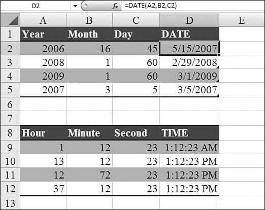
year—This argument can be one to four digits. Ifyearis between 0 and 1899 (inclusive), Excel adds that value to 1900 to calculate the year. For example, =DATE(100,1,2)returnsJanuary 2, 2000(1900+100). If year is between 1900 and 9999 (inclusive), Excel uses that value as the year. For example, =DATE(2000,1,2)returns January 2, 2000. Ifyearis less than 0 or is 10000 or greater, Excel returns a#NUM!error.month—This is a number representing the month of the year. Ifmonthis greater than 12,monthadds that number of months to the first month in the year specified. For example, =DATE(1998,14,2)returns the serial number representing February 2, 1999.day—This is a number representing the day of the month. Ifdayis greater than the number of days in the month specified,dayadds that number of days to the first day in the month. For example, =DATE(1998,1,35)returns the serial number representing February 4, 1998. In a trivial example,=DATE(2007,3,5)returnsMarch 5, 2007.
The true power in the DATE function occurs when one or more of the year, month, or day are calculated values. Here are some examples:
- If Cell A2 contains an invoice date and you want to calculate the day one month later, you use
=DATE(Year(A2),Month(A2)+1,Day(A2)). - To calculate the beginning of the month, you use =
DATE(Year(A2),Month(A2),1). - To calculate the end of the month, you use
=DATE(Year(A2),Month(A2)+1,1)-1.
The DATE function is amazing because it enables Excel to deal perfectly with invalid dates. If your calculations for month causes it to exceed 12, this is no problem. For example, if you ask Excel to calculate =DATE(2006,16,45), Excel considers the 16th month of 2006 to be April 2007. To find the 45th day of April 2007, Excel moves ahead to May 15, 2007.
Figure 23.33 shows various results of the DATE and TIME functions.
Figure 23.33. The formulas in Column D use DATE or TIME functions to calculate an Excel serial number from three arguments.
Using TIME to Calculate a Time
The TIME function is similar to the DATE function. It calculates a time serial number given a specific hour, minute, and second.
Syntax: =TIME(hour,minute,second)
The TIME function returns the decimal number for a particular time. The decimal number returned by TIME is a value ranging from 0 to 0.99999999, representing the times from 0:00:00 (12:00:00 a.m.) to 23:59:59 (11:59:59 p.m.). This function takes the following arguments:
hour—This is a number from0to23, representing the hour.minute—This is a number from0to59, representing the minute.second—This is a number from0to59, representing the second.
As with the DATE function, Excel can handle situations in which the minute or second argument calculates to more than 60. For example, =TIME(12,72,120) evaluates to 1:14 PM.
Additional examples of TIME are shown in the bottom half of Figure 23.33 in the preceding section.
Using DATEVALUE to Convert Text Dates to Real Dates
It is easy to end up with a worksheet full of text dates. Sometimes this is due to importing data from another system. Sometimes it is caused by someone not understanding how dates work.
If your dates are in many conceivable formats, you can use the DATEVALUE function to convert the text dates to serial numbers, which can then be formatted as dates.
Syntax: =DATEVALUE(date_text)
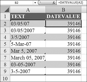
The DATEVALUE function returns the serial number of the date represented by date_text. You use DATEVALUE to convert a date represented by text to a serial number. The argument date_text is text that represents a date in an Excel date format. For example, "1/30/1998" and "30-Jan-1998" are text strings within quotation marks that represent dates. Using the default date system in Excel for Windows, date_text must represent a date from January 1, 1900, to December 31, 9999. DATEVALUE returns a #VALUE! error if date_text is out of this range. If the year portion of date_text is omitted, DATEVALUE uses the current year from your computer’s built-in clock. Time information in date_text is ignored.
Any of the text values in Column A of Figure 23.34 are successfully translated to a date serial number. In this instance, Excel should have been smart enough to automatically format the resulting cells as dates. By default, the cells are formatted as numeric. This leads many people to believe that DATEVALUE doesn’t work. You have to apply a date format in order to achieve the desired result.
Figure 23.34. The formulas in Column B use DATEVALUE to convert the text entries in Column A to date serial numbers.
Caution
The DATEVALUE function must be used with text dates. If you have a column of values in which some values are text and some are actual dates, using DATEVALUE on the actual dates will cause a #VALUE error.
Using TIMEVALUE to Convert Text Times to Real Times
It is easy to end up with a column of text values that look like times. Similarly to DATEVALUE, you can use the TIMEVALUE function to convert these to real times.
Syntax: =TIMEVALUE(time_text)
The TIMEVALUE function returns the decimal number of the time represented by a text string. The decimal number is a value ranging from 0 to 0.99999999, representing the times from 0:00:00 (12:00:00 a.m.) to 23:59:59 (11:59:59 p.m.). The argument time_text is a text string that represents a time in any one of the Microsoft Excel time formats. For example, "6:45 PM" and "18:45" are text strings within quotation marks that represent time. Date information in time_text is ignored.
The TIMEVALUE function is difficult to use because it is easy for a person to enter the wrong formats. In Figure 23.35, many people would interpret Cell A8 as meaning 45 minutes and 30 seconds. Excel, however, treats this as 45 hours and 30 minutes. This misinterpretation makes TIMEVALUE almost useless for a column of cells that contain a text representation of minute and seconds. (The “Excel Troubleshooting” section later in this chapter discusses how to solve this.)
Figure 23.35. The formulas in Column B use TIMEVALUE to convert the text entries in Column A to times. If there is not a leading zero before entries with minutes and seconds, the formula produces an unexpected result.

Frustratingly, Excel does not automatically format the results of this function as a time. Column B shows the result as Excel presents it. Column C shows the same result after a time format has been applied.
Using WEEKDAY to Group Dates by Day of the Week
The WEEKDAY function would not be so intimidating if people could just agree how to number the days. This one function can give three different results.
Syntax: =WEEKDAY(serial_number,return_type)
The WEEKDAY function returns the day of the week corresponding to a date. The day is given as an integer, ranging from 1 (Sunday) to 7 (Saturday), by default. This function takes the following arguments:
serial_number—This is a sequential number that represents the date of the day you are trying to find. Dates may be entered as text strings within quotation marks (for example,"1/30/1998","1998/01/30"), as serial numbers (for example,35825, which represents January 30, 1998), or as results of other formulas or functions (for example,DATEVALUE("1/30/1998")).return_type—This is a number that determines the type of return value:• If
return_typeis1or omitted,WEEKDAYworks like the calendar on your wall. Typically, calendars are printed with Sunday on the left and Saturday on the right. The default version ofWEEKDAYnumbers these columns from 1 through 7.• If
return_typeis2, you are using the biblical version ofWEEKDAY. In the biblical version, Sunday is the seventh day. Working backward, Monday must occupy the 1 position.• If
return_typeis3, you are using the accounting version ofWEEKDAY. In this version, Monday is assigned a value of0, followed by1for Tuesday, and so on. This version makes it very easy to group records by week. If Cell A2 contains a date, thenA2-WEEKDAY(A2,3)converts the date to the Monday that starts the week.
Figure 23.36 shows the results of WEEKDAY for all three return types.
Figure 23.36. Columns B, C, and D compare the WEEKDAY function for the three different return_type values shown in Row 3.

Using WEEKNUM to Group Dates into Weeks
WEEKNUM is a disappointing function. It is disappointing because Microsoft does not perform the function correctly. Microsoft is probably keeping the calculation consistent with some earlier spreadsheets that started doing this incorrectly. However, it would be really easy for Microsoft to add a new pair or return_type arguments that would calculate WEEKNUM correctly.
Syntax: =WEEKNUM(serial_num,return_type)
The WEEKNUM function returns a number that indicates where the week falls numerically within a year. This function takes the following arguments:
serial_num—This is a date within the week.return_type—This is a number that determines on what day the week begins. The default is1. Ifreturn_typeis1or omitted, the week begins on Sunday. Ifreturn_typeis2, the week begins on Monday.
Figure 23.37 shows WEEKNUM for the first eight days of each year of the next eight years. Rows 13 through 20 show WEEKNUM with a return_type of 1, so the week starts on Sunday.
Figure 23.37. Excel calculates week numbers, but they are out of sync with the rest of the world.
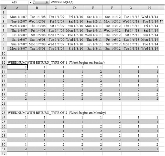
Look at Column F. The first day of the year is a Sunday. This works; Cells F13:F19 report the first seven days as Week 1, and Cell F20 reports Sunday, January 8, 2012, as the first “day of the” week for Week 2.
However, look at E13:E20. In this case, the year 2011 starts on a Saturday. The first day of the year is treated as Week 1. Excel says that Week 2 starts on January 2, 2010. It is horrible to have a one-day week starting your year. It guarantees that you will have a significant Week 53 at the end of the year.
There is an ANSI standard for week numbering. This system says that your Week 1 must have at least four days. In the ANSI system, Saturday, January 1, 2011, would be called Week 0. In this system, whichever week contains January 4 is considered Week 1.
Alternate Calendar Systems and DAYS360
There are many alternate calendar systems that you might have to work with in Excel. Here are some examples:
- Manufacturers often redefine a quarter as being composed of 13 workweeks, with the first 4 weeks being called Month 1, the next 4 weeks being Month 2, and the final 5 weeks being Month 3. This is known as a 4-4-5 calendar.
- Retailers use a special retail calendar composed of 52 7-day weeks. Each week ends on a Sunday. If you compare Week 7, Day 6 of one year to Week 7, Day 6 of another year, you are assured that you are comparing a Saturday to a Saturday and can have a like comparison.
- Some accounting systems use a 360-day calendar. In this type of system, the year is divided into 12 months of 30 days. There is special handling for months with 31 days. Unfortunately, U.S. and European accounting boards disagree on the special handling, so there are two sets of rules.
Out of these three alternate calendar systems, Excel handles only the 360-day calendar. Excel provides the DAYS360 function and the YEARFRAC function to deal with the date system.
Syntax: =DAYS360(start_date,end_date,method)
The DAYS360 function returns the number of days between two dates, based on a 360-day year (12 30-day months), which is used in some accounting calculations. You use this function to help compute payments if your accounting system is based on 12 30-day months. This function takes the following arguments:
start_dateandend_date—These are the two dates between which you want to know the number of days. Ifstart_dateoccurs afterend_date,DAYS360returns a negative number. Dates may be entered as text strings within quotation marks (for example,"1/30/1998","1998/01/30"), as serial numbers (for example,35825, which represents January 30, 1998, if you’re using the 1900 date system), or as results of other formulas or functions (for example,DATEVALUE("1/30/1998")).method—This is a logical value that specifies whether to use the U.S. or European method in the calculation:•
FALSEor omitted is a U.S. (National Association of Securities Dealers) method. If the starting date is the 31st of a month, it becomes equal to the 30th of the same month. If the ending date is the 31st of a month and the starting date is earlier than the 30th of a month, the ending date becomes equal to the 1st of the next month; otherwise, the ending date becomes equal to the 30th of the same month.•
TRUEis a European method. Starting dates or ending dates that occur on the 31st of a month become equal to the 30th of the same month.
Using YEARFRAC or DATEDIF to Calculate Elapsed Time
If you work in a human resources department, you might be concerned with years of service in order to calculate a certain benefit. Excel provides one function, YEARFRAC, that can calculate decimal years of service in five different ways. An old function, DATEDIF, has been hanging around since Lotus 1-2-3; it can calculate the difference between two dates in complete years, months, or days.
Syntax: =YEARFRAC(start_date,end_date,basis)
The YEARFRAC function calculates the fraction of the year represented by the number of whole days between two dates (start_date and end_date). You use the YEARFRAC worksheet function to identify the proportion of a whole year’s benefits or obligations to assign to a specific term.
This function takes the following arguments:
start_date—This is a date that represents the start date. Dates may be entered as text strings within quotation marks (for example,"1/30/1998","1998/01/30"), as serial numbers (for example,35825, which represents January 30, 1998, if you’re using the 1900 date system), or as results of other formulas or functions (for example,DATEVALUE("1/30/1998")).end_date—This is a date that represents the end date.basis—This is the type of day count basis to use. Figure 23.38 compares the five types ofbasisavailable:• If
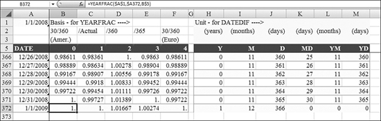
basisis0or omitted, Excel uses a 30/360 plan, modified for American use. In this plan, the employee earns 1/360 of a year’s credit on most days. The employee earns no service on the day after any 31st of the month. In a leap year, the employee earns 2/360 of a year for showing up on March 1. In a non–leap year, the employee earns 3/360 of a year for showing up on March 1.• If
basisis1, the actual number of elapsed days is divided by the actual number of days in the year. This method works well and ensures that the year fraction ends up being1on the anniversary date, whether it is a leap year or not.• If
basisis2, the actual number of elapsed days is divided by 360. If someone would show up and work for 30 years straight for one employer, this method would give that person an extra 0.4528 years of credit. Sisogenes would be spinning in his grave.• If
basisis3, the actual number of elapsed days is divided by 365. This works great for three out of every four years. It is slightly wrong in leap years.• If
basisis4, Excel uses a 30/360 plan, modified for European use. This is similar to the defaultbasisof0. In this plan, the employee gets no credit for working any 31st of the month. The employee still gets triple credit for working March 1 (to make up for the 29th and 30th of February). In a leap year, March 1 is worth only double credit.
Figure 23.38. If your benefits package includes information about complete months, then YEARFRAC with a basis value of 0 works best. Otherwise, a basis value of 1 is the most accurate.
Syntax: =DATEDIF(start_date,end_date,unit)
In contrast to YEARFRAC, the DATEDIF function calculates complete years, months, or days. This function calculates the number of days, months, or years between two dates. It is provided for compatibility with Lotus 1-2-3. This function takes the following arguments:
start_date—This is a date that represents the first, or starting, date of the period. Dates may be entered as text strings within quotation marks (for example,"2001/1/30"), as serial numbers, or as the results of other formulas or functions (for example,DATEVALUE("2001/1/30")).end_date—This is a date that represents the last, or ending, date of the period.unit—This is the type of information you want returned. The various values forunitare shown in Table 23.5.
Table 23.5. unit Values Used by the DATEDIF Function
Figure 23.38 compares the five types of basis of YEARFRAC with the six unit values of DATEDIF. Each cell uses $A$1 as the start date and that row’s Column A as the end date.
Using EDATE to Calculate Loan or Investment Maturity Dates
If someone invests in a six-month CD on the 17th of the month, the maturity date is on the 17th of another month. This would be a fairly straightforward calculation if no one invested on the 31st of a month.
The maturity rules work such that if you invest on the 31st of a month, and the CD would be scheduled to mature on the 31st of June, the CD maturity actually happens on the last day of June, which is June 30.
If a CD is to mature on the 31st, 30th, or 29th day of February, the CD matures on the last day of February.
Syntax: =EDATE(start_date,months)
The EDATE function returns the serial number that represents the date that is the indicated number of months before or after a specified date (that is, start_date). You use EDATE to calculate maturity dates or due dates that fall on the same day of the month as the date of issue. This function takes the following arguments:
start_date—This is a date that represents the start date. Dates may be entered as text strings within quotation marks (for example,"1/30/1998","1998/01/30"), as serial numbers (for example,35825, which represents January 30, 1998, if you’re using the 1900 date system), or as results of other formulas or functions (for example,DATEVALUE("1/30/1998")). If thestart_dateis not valid,EDATEreturns a#NUM!error.months—This is the number of months before or afterstart_date. A positive value formonthsyields a future date; a negative value yields a past date. Ifmonthsis not an integer, it is truncated.
Figure 23.39 shows several examples of EDATE. Note that in Column B, the function is a no-brainer. You could easily calculate it by using the DATE function. The only interesting cases occur on the 29th, 30th, and 31st of the month.
Figure 23.39. You can use EDATE to calculate the maturity date for a security.

Note that EDATE can be used to back into an investment date from a maturity date. For example, the records in Rows 11 through 16 pass a negative number for the months parameter.
Caution
You have to format the result of the EDATE formula to be a date to see the expected results.
Using EOMONTH to Calculate the End of the Month
Before Excel 2007, about 89 functions were available only in the Analysis Toolpack. Some companies had rules that you were not allowed to build spreadsheets using the functions in the Analysis Toolpack. This rule was probably created by some corporate executive who didn’t know how to turn on the Analysis Toolpack!
One of my favorite puzzles at MrExcel.com came from someone who worked at such a company. How can you calculate the end of the month without using EOMONTH? This is a hard question; the end of the month is the 31st if the month number is 1, 3, 5, 7, 8, 10, or 12. It is the 30th if the month number is 4, 6, 9, or 11. If the month number is 2, then you have to look at the year to figure out if it is a leap year for 29 days or not a leap year for 28 days. The formula to solve this was horrible:
=DATE(YEAR(A2),MONTH(A2),CHOOSE(MONTH(A2),31,28,31,30,31,30,31,31,30,31,30,31)
+IF(MOD(YEAR(A2),4)=0,1,0))
Well-known Excel guru Aladin Akyurek weighed in with the great answer and ended the entire discussion. Aladin suggested using the DATE function to move up to the first of the next month and then simply subtract one day, using this formula:
=DATE(YEAR(A2),MONTH(A2)+1,1)-1
The sheer simplicity of this is beautiful. However, the whole question becomes immaterial now that EOMONTH has been promoted to be part of the actual Excel function set.
Syntax: =EOMONTH(start_date,months)
The EOMONTH function returns the serial number for the last day of the month that is the indicated number of months before or after start_date. You use EOMONTH to calculate maturity dates or due dates that fall on the last day of the month. This function takes the following arguments:
start_date—This is a date that represents the starting date. Dates may be entered as text strings within quotation marks (for example,"1/30/1998","1998/01/30"), as serial numbers, or as results of other formulas or functions (for example,DATEVALUE("1/30/1998")). Ifstart_dateis not a valid date,EOMONTHreturns a#NUM!error.months—This is the number of months before or afterstart_date. A positive value formonthsyields a future date; a negative value yields a past date. Ifmonthsis not an integer, it is truncated. Ifstart_dateplusmonthsyields an invalid date,EOMONTHreturns a#NUM!error.
=EOMONTH(A2,0) converts any date to the end of the month.
Caution
You have to format the result of the EOMONTH formula to be a date to see the expected results.
Using WORKDAY or NETWORKDAYS to Calculate Workdays
If you work in a service industry, allow me to apologize to you on behalf of Microsoft. If you work in retail, this section won’t work for you. If you are in one of the countries where you have every Thursday off, this will not work. The workday functions work only for those people who still work in a traditional Monday-through-Friday work environment.
If you happen to be in a Monday-through-Friday environment, the functions WORKDAY and NETWORKDAYS are pretty cool. For example, they are great for calculating shipping days when you ship with FedEx or UPS. It takes a little work to get the holidays set up with these functions. Here’s how you do it:
- In an out-of-the-way section of a spreadsheet, enter any holidays that will fall during the workweek. This might be federal holidays, floating holidays, company holidays, and so on. The list of holidays can either be entered down a column or across a row. In the top portion of Figure 23.40, the holidays are in E2:E7.
Figure 23.40.
WORKDAYandNETWORKDAYcan calculate the number of Monday-through-Friday days, exclusive of a range of holidays.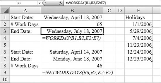
- Enter a starting date in a cell, such as B1.
- Enter the number of workdays that the project is expected to take in another cell, such as B2.
- Enter the ending date formula as
=WORKDAY(B1,B2,E2:E7).
The NETWORKDAYS function takes two dates and figures out the number of workdays between them. For example, you might have a project that is due on June 18, 2007. If today is April 14, 2007, NETWORKDAYS can calculate how many workdays there are until the project is due.
Syntax: =NETWORKDAYS(start_date,end_date,holidays)
The NETWORKDAYS function returns the number of whole workdays between start_date and end_date. Workdays exclude weekends and any dates identified in holidays. You use NETWORKDAYS to calculate employee benefits that accrue based on the number of days worked during a specific term. This function takes the following arguments:
start_date—This is a date that represents the start date. Dates may be entered as text strings within quotation marks (for example,"1/30/1998","1998/01/30"), as serial numbers, or as results of other formulas or functions (for example,DATEVALUE("1/30/1998")).end_date—This is a date that represents the end date.holidays—This is an optional range of one or more dates to exclude from the working calendar, such as state and federal holidays and floating holidays. The list can be either a range of cells that contain the dates or an array constant of the serial numbers that represent the dates. If any argument is not a valid date,NETWORKDAYSreturns a#NUM!error.
In Figure 23.40, the current date is entered in Cell B6. The project due date is entered in Cell B7. The holidays range is in E2:E7, as in the previous example. The formula in Cell B8 to calculate workdays is =NETWORKDAYS(B6,B7,E2:E7).
Excel in Practice: Converting a Holiday Range to an Array
The problem with putting the list of holidays in a range on a worksheet is that someone might accidentally overwrite or change the range of holidays.
The syntax for the workdays functions mentions that the holiday range can be converted to an array of serial numbers. To embed the holidays inside a function, you follow these steps:
- In Figure 23.40, select cell B3.
- In the Formula Bar, use the mouse to select the characters E2:E7.
- Press the F9 key. Excel will replace the selected characters with the calculated version of those characters. In this case, the calculation is the array {38718,38866,etc.} as shown in Figure 23.41.
Figure 23.41. You can remove the holiday cells from the worksheet after embedding the array in the formula.

- Press Enter to accept the new formula.
- You can now delete the holidays in column E.
Examples of Text Functions
When they think of Excel, most people think of numbers. Excel is great at dealing with numbers, and it lets you write formulas to produce new numbers. Excel offers a whole cadre of formulas for dealing with text.
You might sometimes be frustrated because you receive data from other users and the text is not in the format you need. Or, the mainframe might send customer names in uppercase, or the employee in the next department might put a whole address in a single cell. Excel provides text functions to deal with all these situations and more.
Joining Text with the Ampersand (&) Operator
Chapter 20, “Formula Basics,” mentions the ampersand (&) operator, but it is worth mentioning again here because it is the most important tool for dealing with text. The & is an operator that you use to join text.
Say that you have a worksheet with first name in Column A and last name in Column B, as shown in Figure 23.42. You need to put these names together in a single cell. If you use the formula =A2&B2 in Cell C2, Excel smashes the names together (for example, STEVENWOODWARD). Instead, you have to join three elements. In between A2 and B2, you need to join a single space in double quotes. The formula to do this is =A2&" "&B2.
Figure 23.42. The & character can be used to join text in cells or text enclosed in quotes.
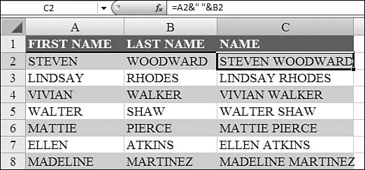
If you only want to keep the data in Column C, you have to convert the formulas to values before deleting Columns A and B. To do this, you select the data in Column C and then press Ctrl+C to copy. Then you select Home, Paste, Paste Values to convert the formulas to values.
Some people prefer to use the CONCATENATE function instead of the &. This function does not perform the way that I want it to perform, and I generally avoid it, but it is described in the following section.
Syntax: =CONCATENATE (text1,text2,...)
The CONCATENATE function joins several text strings into one text string. The arguments text1, text2,... are 1 to 30 text items to be joined into a single text item. The text items can be text strings, numbers, or single-cell references.
The problem with this function is that it can only select single cell references. An attempt to use =CONCATENATE(A2:B2) returns a #VALUE! error. If you have to enter =CONCATENATE(A2," ",B2), it is easier to use =A2&" "&B2. Further, the function can handle only 30 references. If you are joining cells with spaces in between, you will run out of terms after just 15 cells. With the &, you can join more than 30 items.
Using LOWER, UPPER, or PROPER to Convert Text Case
Three functions—LOWER, UPPER, and PROPER—convert text to or from capital letters. In Figure 23.43, the products in Column A were entered in a haphazard fashion. Some products used lowercase, and some products used uppercase. Column B uses =UPPER(A2) to make all the products a uniform uppercase.
Figure 23.43. UPPER, LOWER, and PROPER can convert text to and from capital letters.

In Cell E13, text was entered by someone who never turns off Caps Lock. You can convert this uppercase to lowercase with =LOWER(E13).
Note
It would be great if Microsoft would add a function to convert to sentence case. We can hope that they add such a function in future versions of Excel.
In Column E, you see a range of names in uppercase. You can use =PROPER(E2) to convert the name to proper case, which capitalizes just the first letter of each word. The PROPER function is mostly fantastic, but there are a few cells that you have to manually correct. PROPER does correctly capitalize names with apostrophes, such as O’Rasi in Cell F3. It does not, however, correctly capitalize the interior c in McCartney in Cell F4. The function is also notorious for creating company names such as Ibm, 3m, and Aep.
Syntax: =LOWER(text)
The LOWER function converts all uppercase letters in a text string to lowercase. The argument text is the text you want to convert to lowercase. LOWER does not change characters in text that are not letters.
Syntax: =PROPER(text)
The PROPER function capitalizes the first letter in a text string and any other letters in text that follow any character other than a letter. It converts all other letters to lowercase letters.
The argument text is text enclosed in quotation marks, a formula that returns text, or a reference to a cell containing the text you want to partially capitalize.
Syntax: =UPPER(text)
The UPPER function converts text to uppercase. The argument text is the text you want converted to uppercase. text can be a reference or text string.
Using TRIM to Remove Trailing Spaces
If you frequently import data, you might be plagued with a couple of annoying situations. This section and the next one deal with those situations.
You may have trailing spaces at the end of text cells. Although "ABC" and "ABC " might look alike when viewed in Excel, they cause functions such as MATCH and VLOOKUP to fail. TRIM removes leading and trailing spaces.
In Figure 23.44, you have a simple VLOOKUP in Column B. The formula in Cell B2 is =VLOOKUP(A2,$F$2:$G$5,2,FALSE). Even though you can clearly see that M40498 is in the lookup table, VLOOKUP returns an #N/A! error, indicating that the product ID is missing from the lookup table.
Figure 23.44. This VLOOKUP should work, but in this instance, it fails.
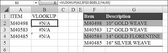
To diagnose and correct this problem, you follow these steps:
- Select one of the data cells in Column F. Press the F2 key to put the cell in Edit mode. A flashing insertion character appears at the end of the cell. Check to see if the flashing cursor is immediately after the last character.
- Select one of the data cells in Column A. Press the F2 key to put the cell in Edit mode. Note whether the flashing insertion character is immediately after the last character. Figure 23.45 shows that the products in Column A have several trailing spaces after them. The products in the lookup table do not have any trailing spaces.
Figure 23.45. Spaces are padding the right side of the products in Column A.

- If the problem is occurring in the values being looked up, you could simply modify the formula in Cell B2 to use the
TRIMfunction. The new formula would be=VLOOKUP(TRIM(A2),$F$2:$G$5,2,FALSE). Figure 23.46 shows how this solves the problem.Figure 23.46. Using
TRIMto remove leading spaces allowsVLOOKUPto work.
- If the problem is occurring in the first column of the lookup table, insert a new temporary column. Enter the function
=TRIM(F2) in the temporary column. Copy this formula down to all rows of the lookup table. Copy the new formulas and select Home, Paste, Values to paste the new values. Although the old and new values look the same, theTRIMfunction has removed the trailing spaces and now the products match.
Syntax: =TRIM(text)
The TRIM function removes all spaces from text except for single spaces between words. You use TRIM on text that you have received from another application that may have irregular spacing. The argument text is the text from which you want spaces removed.
In Figure 23.47, Cell C1 contains six letters: ABC DEF. You might assume that the cell is set to be centered. However, the formula in Cell C2 appends an asterisk to each end of the value in Cell C1. This formula shows that there are several leading and trailing spaces in the value.
Figure 23.47. TRIM removes leading spaces and extra interior spaces.

Using =LEN(C1) shows that the text actually contains 15 characters instead of 6 characters. The TRIM(C1) formula removes any leading spaces, any trailing spaces, and any extra interior spaces. The function still leaves one space between ABC and DEF because you want to continue to have words separated by a single space.
The formulas in Cells C5 and C6 confirm that the leading and trailing spaces are removed and that the length of the new value is only seven characters.
Using CLEAN to Remove Nonprintable Characters from Text
Although TRIM works great, the CLEAN function no longer works as advertised. CLEAN is designed to remove nonprintable characters from text.
Besides extra spaces, another annoying problem with data from other systems is that it may contain nonprintable characters. Excel offers a function that is supposed to remove nonprintable characters, but Microsoft’s definition of a nonprintable character is far too narrow. The function was clearly written before the proliferation of web queries, Oracle, and SAP.
Syntax: =CLEAN(text)
The CLEAN function removes all nonprintable characters from text. You use CLEAN on text imported from other applications that contains characters that may not print with your operating system. For example, you can use CLEAN to remove some low-level computer code that is frequently at the beginning and end of data files and cannot be printed.
The argument text is any worksheet information from which you want to remove nonprintable characters.
Unfortunately, Microsoft’s definition of nonprintable characters is limited to the “old-time” bad characters. Today, you are likely to encounter far more bad characters than those.
Figure 23.48 shows data in Column A with characters that I routinely find in imported data. You might expect the CLEAN function in Column B to fix all these problems. If so, you will be highly disappointed. In the first pass, CLEAN did not clean any of the bad characters. After I edited Cell A2 to use a traditional nonprintable character, Cell B2 was able to clean that one character.
Figure 23.48. CLEAN removes a short list of nonprintable characters. Unfortunately, today’s data is littered with a new crop of nonprintable characters.
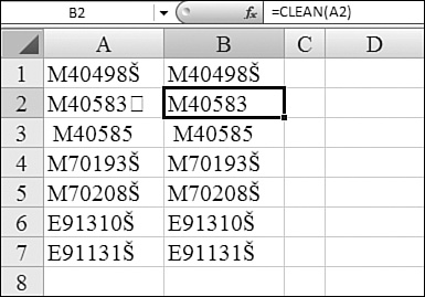
To figure out exactly how CLEAN works, you need the CHAR function, which is conveniently scheduled to be discussed next. Read on for more of the CLEAN saga.
Using the CHAR Function to Generate Any Character
Computers have the ability to display 255 different characters in any given font. For the past 20 years, this set of 255 characters has been known as the ASCII (pronounced “ask-key”) character set. My U.S. keyboard gives me the ability to type 96 of those characters. The keyboard in another country may offer several more or fewer characters, but the point is that you cannot access all 255 characters by using your keyboard.
You might have ventured into Start, All Programs, Accessories, System Tools, Character Map in order to find a particular character in the Wingdings character set. Also, if you have a favorite symbol, you might have memorized that you can insert the symbol by using a hotkey. For example, if you hold down Alt, type 0169 on the numeric keypad, and then release Alt, an Office program inserts the copyright symbol (©).
In Excel, rather than use hotkeys and the character map, you can use the CHAR function to generate a specific character.
Syntax: =CHAR(number)
The CHAR function returns the character specified by a number. You use CHAR to translate code page numbers you might get from files on other types of computers into characters.
The argument number is a number between 1 and 255 that specifies which character you want. The character is from the character set used by your computer.
Although I know a few characters off the top of my head, I usually take a look at all characters in a set by entering =CODE(ROW()) in Cells A1:A255. This returns Character 65 in Row 65, and so on.
To figure out which characters were actually removed by the CLEAN function (refer to the preceding section), I built a table with the numbers from 1 through 255. In Figure 23.49, Column A contains the character number. Column B has the function =CHAR(A2) to display that character in the Times New Roman font. Column C has a formula to reveal whether CLEAN removes that character: =IF(LEN(CLEAN(B2))=0,"YES","NOT). After you copy these formulas to all 255 rows, you will learn that CLEAN removes characters numbered 1 through 31, 129, 141, 144, and 157.
Figure 23.49. This figure shows all CHAR values in the Times New Roman dataset. Only the characters highlighted in black are removed by CLEAN.

To fit in one screen of cells, Figure 23.49 shows all the codes arranged on one page.
If you see a strange character in your data, you can learn the character number by using the CODE function, as described in the following section.
Using the CODE Function to Learn the Character Number for Any Character
Each font set offers 255 different characters, numbered from 1 through 255. Old-time computer folks might know some of the popular codes off the top of their heads. For example, a capital A is 65. The capital letters run from 65 to 90, a space is 32, a lowercase letter a is 97, and the other lowercase letters run from 97 through 122.
In the early days of personal computers, every computer was packed with a list of the ASCII codes for each character. Today, with the character map, no one has to memorize character codes. However, in some instances, you might want to learn exactly what character you are seeing in a cell. The CODE function returns the character code for one character at a time.
Syntax: =CODE(text)
The CODE function returns a numeric code for the first character in a text string. The returned code corresponds to the character set used by your computer. The argument text is the text for which you want the code of the first character. This is an important distinction. CODE returns the code for only the first character in a cell. =CODE("A") and =CODE("ABC") return only 65 to indicate the capital letter A.
A new problem began happening in Excel in the past few years. People started encountering values with which TRIM would not remove the spaces from the text. For example, Figure 23.50 shows a value in Column A that very clearly contains several spaces in between the letters A and B.
Figure 23.50. CODE is instrumental in learning why the TRIM function won’t work on the data in Column A.

Excel pros know that they could remove the extra interior spaces by using =TRIM(A2). But if you look at the formula in Cell B2, you see that TRIM is not removing the interior spaces. This requires some additional investigation, and CODE is the key to solving the problem. Because CODE can work on only the first character in a cell, formulas in Columns C and D isolate each character in the text. (For details on this, see the section “Syntax: MID(text,start_num,num_chars),” later in this chapter).
The CODE(D2) formula in Column E shows the character number for each character in the text. Things start out well enough, with a character 65 being returned for the A. They also end up okay, with a character 66 being returned for the B at the end in Row 9. However, all the middle characters are returning a character 160 instead of a typical space—character 32.
If you’ve ever created a small webpage, you might have learned that browsers ignore consecutive spaces. If you really want to keep two words separated by four spaces, you need to use Word1 Word2. I learned this trick somewhere on the Web and never really thought about what means. It turns out that it is a nonbreaking space. And, you guessed it, a nonbreaking space occupies character position 160, so it looks just like a space. Web designers use it all the time to format webpages. Consequently, it is ending up in data that people paste into Excel from the Web, and it is making it appear that TRIM does not always work.
Note
To actually remove nonbreaking space characters, you have to use the SUBSTITUTE function, discussed in the section “Using SUBSTITUTE and REPLACE to Replace Characters,” later in this chapter.
Using LEFT, MID, or RIGHT to Break Text
One of the newer rules in information processing is that each field in a database should contain exactly one piece of information. Throughout the history of computers, there have been millions of examples of people trying to cram many pieces of information into a single field.
Although this works great for humans, it is pretty difficult to have Excel to sort a column by everything in the second half of a cell.
Column A in Figure 23.51 contains part numbers. As you might guess, the Part Number field really contains two pieces of information: a three-character vendor code, a dash, and a five-digit part number.
Figure 23.51. LEFT makes quick work of extracting the vendor code. Several varieties of MID or RIGHT extract the part number.
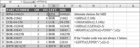
When a customer comes in to buy a part, he probably doesn’t care about the vendor. So the real question is “Do you have anything in stock that can fix my problem?”
Excel offers three functions—LEFT, MID, and RIGHT—that allow you to isolate just the first or just the last characters, or even just the middle characters, from a column.
Syntax: =LEFT(text,num_chars)
The LEFT function returns the first character or characters in a text string, based on the number of characters specified. This function takes the following arguments:
text—This is the text string that contains the characters you want to extract.num_chars—This specifies the number of characters you wantLEFTto extract.num_charsmust be greater than or equal to zero. Ifnum_charsis greater than the length of text,LEFTreturns all oftext. Ifnum_charsis omitted, it is assumed to be1.
Syntax: =RIGHT(text,num_chars)
The RIGHT function returns the last character or characters in a text string, based on the number of characters specified. This function takes the following arguments:
text—This is the text string that contains the characters you want to extract.num_chars—This specifies the number of characters you wantRIGHTto extract.num_charsmust be greater than or equal to zero. Ifnum_charsis greater than the length of text,RIGHTreturns all oftext. Ifnum_charsis omitted, it is assumed to be1.
Syntax: =MID(text,start_num,num_chars)
MID returns a specific number of characters from a text string, starting at the position specified, based on the number of characters specified. This function takes the following arguments:
text—This is the text string that contains the characters you want to extract.start_num—This is the position of the first character you want to extract in text. The first character in text hasstart_num1, and so on. Ifstart_numis greater than the length of text,MIDreturns""(that is, empty text). Ifstart_numis less than the length of text, butstart_numplusnum_charsexceeds the length of text,MIDreturns the characters up to the end of text. Ifstart_numis less than1,MIDreturns a#VALUE!error.num_chars—This specifies the number of characters you wantMIDto return from text. Ifnum_charsis negative,MIDreturns a#VALUE!error.
In Figure 23.51, it is easy to extract the three-digit vendor code by using =LEFT(A2,3). It is a bit more difficult to extract the part number. As you scan through the values in Column A, it is clear that the vendor code is consistently three letters. With the dash in the fourth character of the text, that means that the part number starts in the fifth position. If you are using MID, you therefore use 5 as the start_num argument.
However, there are a few thousand part numbers in the dataset. Right up front, in Cell A4, is a part number that breaks the rule. LUK-04-158 contains six characters after the dash. This might seem to be an isolated incident, but in Row 10, BWW-BC42TW also contains six characters after the dash. Because this type of thing happens in real life, two errors in the first nine records are enough to warrant a little extra attention. The four possible strategies for extracting the part number are listed in G2:G6. They are:
- Ask
MIDto start at the fifth character and return a large enough number of characters to handle any possible length (that is,=MID(A2,5,100)). - Ask
MIDto start at the fifth character but useTRIMaround the whole function to prevent any trailing spaces from being included (that is,=TRIM(MID(A2,5,100))). - Ask
MIDto start at the fifth character, but calculate the exact number of characters by using theLENfunction (that is,=MID(A2,5,LEN(A2)-4)). - Skip
MIDaltogether and askRIGHTto return all the characters after the first dash. This requires you to use theFINDfunction to locate the first dash (that is,=RIGHT(A2,LEN(A2)-FIND("-",A2))).
Using LEN to Find the Number of Characters in a Text Cell
It seems pretty obscure, but you will find the LEN function amazingly useful. The LEN function determines the length of characters in a cell, including any leading or trailing spaces.
Syntax: =LEN(text)
The LEN function returns the number of characters in a text string. The argument text is the text whose length you want to find. Spaces count as characters.
There are instances in which LEN can be used in conjunction with LEFT, MID, or RIGHT to isolate a portion of text. (Refer to the example in the previous section.)
LEN can also be used to find records that are longer than a certain limit. Say you are about to order nameplates for company employees. Each nameplate can accommodate 15 characters. In Figure 23.52, you add the LEN function next to the names and sort by the length, in descending order. Any problem names appear at the top of the list.
Figure 23.52. LEN identifies the number of characters in a cell.
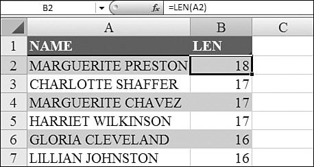
Using SEARCH or FIND to Locate Characters in a Particular Cell
Two nearly identical functions can scan through a text cell, looking for a particular character or word. Many times, you just want to know if the word appears in the text. These functions go further than telling you if the character exists in the text; they tell you at exactly which character position the character or word is found. The character position can be useful in subsequent formulas with LEFT, RIGHT, or REPLACE.
First, let’s look at an example of using FIND to determine whether a word exists in another cell. Figure 23.53 shows a database of customers. The database was created by someone who doesn’t know Excel and jammed every field into a single cell.
Figure 23.53. When the manager asked an employee to type this in Excel, she didn’t realize that the employee had never used Excel before.

Note
Like all the other datasets in this book, these names and addresses are randomly generated from lists of the most popular first name, last name, street name, and city names. Don’t try to send Christmas cards to these people as none of the addresses actually exist. And don’t think that the zip codes are real; everything here is completely random.
Here is how to make this work properly:
- To find all the customers in California, in Cell B2, enter
=FIND(", CA",A2). When you enter the formula, you get a#VALUE!error. This is okay. In fact, it is useful information: It tells you thatCAis not found in the first record. - Copy the formula down to all rows.
- Sort low to high by Column B. 98% of the records have a
#VALUE!error and sort to the bottom of the list. The few California records have a valid result for the formula in Column B and sort to the top of the list, as shown in Figure 23.54.
Figure 23.54. You don’t care where FIND found the text; you simply want to divide the list into records with valid values versus errors.

Caution
The trick with this application of FIND is to look for something that is only likely to be found in California records. If you had customers in Cairo, Illinois, they would have also been found by the FIND command you just used. The theory with this sort of search is that you can quickly check through the few matching records to find false positives.
FIND and SEARCH are similar to one another. The FIND function does not distinguish between uppercase and lowercase letters. FIND identifies CA, ca, Ca, and cA as matches for CA. If you need to find a cell with exactly AbCdEf, you need to use the SEARCH command instead of FIND. Also, SEARCH allows for wildcard characters in find_text. A question mark (?) finds a single character, and an asterisk (*) finds any number of characters.
The FIND function makes it easy to find the first instance of a particular character in a cell. However, if your text values contain two instances of a character, your task is a bit more difficult. In Figure 23.55, the part numbers in Column A really contain three segments, each separated by a dash:
- To find the first dash, enter
=FIND("-",A2)in Column B. - To find the second dash, use the optional
start_numparameter to theFINDfunction. Thestart_numparameter is a character position. You want the function to start looking after the first instance of a dash. This can be calculated as the result of the firstFINDin Column B plus one. Thus, the formula in cell C2 is=FIND("-",A2,B2+1). - After you find the character positions of the dashes, isolate the various portions of the part number. In Column D, for the first part of the number, enter
=LEFT(A2,B2-1). This basically asks for the left characters from the part number, stopping at one fewer than the first dash. - In Column E, for the middle part of the number, enter
=MID(A2,B2+1,C2-B2-1). This asks Excel to start at the character position one after the first dash and then continue for a length that is one fewer than the first dash subtracted from the second dash. - In Column F, for the final part of the number, enter
=RIGHT(A2,LEN(A2)-C2). This calculates the total length of the part number, subtracts the position of the second dash, and returns those right characters.
Figure 23.55. Formulaically isolating data between the first and second dashes can be done, but it helps to break each number down into small parts.

Syntax: =FIND(find_text,within_text,start_num)
FIND finds one text string (find_text) within another text string (within_text) and returns the number of the starting position of find_text from the first character of within_text. You can also use SEARCH to find one text string within another, but unlike SEARCH, FIND is case-sensitive and doesn’t allow wildcard characters.
The FIND function takes the following arguments:
find_text—This is the text you want to find. Iffind_textis""(that is, empty text),FINDmatches the first character in the search string (that is, the character numberedstart_numor1).find_textcannot contain any wildcard characters.within_text—This is the text that contains the text you want to find.start_num—This specifies the character at which to start the search. The first character inwithin_textis character number 1. If you omitstart_num, it is assumed to be1.
If find_text does not appear in within_text, FIND return a #VALUE! error. If start_num is not greater than zero, FIND returns a #VALUE! error. If start_num is greater than the length of within_text, FIND return a #VALUE! error.
Syntax: =SEARCH(find_text,within_text,start_num)
SEARCH returns the number of the character at which a specific character or text string is first found, beginning with start_num. You use SEARCH to determine the location of a character or text string within another text string so that you can use the MID or REPLACE functions to change the text.
The SEARCH function takes the following arguments:
find_text—This is the text you want to find. You can use the wildcard characters question mark (?) and asterisk (*) infind_text. A question mark matches any single character; an asterisk matches any sequence of characters. If you want to find an actual question mark or asterisk, you type a tilde (~) before the character. Iffind_textis not found, a#VALUE!error is returned.within_text—This is the text in which you want to search forfind_text.start_num—This is the character number inwithin_textat which you want to start searching. Ifstart_numis omitted, it is assumed to be1. Ifstart_numis not greater than zero or is greater than the length ofwithin_text, a#VALUE!error is returned.
Using SUBSTITUTE and REPLACE to Replace Characters
When you have the ability to find text, you might want to replace text. Excel offers two functions for this: SUBSTITUTE and REPLACE. The SUBSTITUTE function is easier to use and should be your first approach.
Syntax: =SUBSTITUTE(text,old_text,new_text,instance_num)
The SUBSTITUTE function substitutes new_text for old_text in a text string. You use SUBSTITUTE when you want to replace specific text in a text string; you use REPLACE when you want to replace any text that occurs in a specific location in a text string.
The SUBSTITUTE function takes the following arguments:
text—This is the text or the reference to a cell that contains text for which you want to substitute characters.old_text—This is the text you want to replace.new_text—This is the text you want to replaceold_textwith.instance_num—This specifies which occurrence ofold_textyou want to replace withnew_text. If you specifyinstance_num, only that instance ofold_textis replaced. Otherwise, every occurrence ofold_textintextis changed tonew_text.
For example, =SUBSTITUTE("Sales Data","Sales","Cost") would generate "Cost Data".
The SUBSTITUTE function works similarly to a traditional find and replace command. Compared to the SUBSTITUTE function, the REPLACE function is difficult enough to make even an old programmer’s head spin.
Syntax: =REPLACE(old_text,start_num,num_chars,new_text)
REPLACE replaces part of a text string, based on the number of characters specified, with a different text string. This function takes the following arguments:
old_text—This is text in which you want to replace some characters.start_num—This is the position of the character inold_textthat you want to replace withnew_text.num_chars—This is the number of characters inold_textthat you wantREPLACEto replace withnew_text.new_text—This is the text that will replace characters inold_text.
In order to successfully use REPLACE, you have to use functions to determine the location and number of characters to replace. In most circumstances, SUBSTITUTE is easier to use.
Using REPT to Repeat Text Multiple Times
A little-known trick has been around for 20-plus years and still works today. Go to a blank cell. Enter a backslash () and any one character. Excel fills the cell with that character! Enter *, and the cell is filled with asterisks. Make the column wider or less narrow, and the number of asterisks changes to fill the cell.
In Excel, if you use -, Excel repeats the two characters over and over until the cell is filled. Cells in Rows 8 through 11 of Figure 23.56 show various cells that use the backslash trick.
Figure 23.56. The REPT function can be used to calculate a certain number of repeated entries.
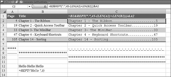
There is an Excel function, REPT, that formalizes this repetition a bit.
Syntax: =REPT(text,number_times)
The REPT function repeats text a given number of times. You use REPT to fill a cell with a number of instances of a text string. This function takes the following arguments:
text—This is the text you want to repeat.number_times—This is a positive number that specifies the number of times to repeat text. Ifnumber_timesis0,REPTreturns""(that is, empty text). Ifnumber_timesis not an integer, it is truncated. The result of theREPTfunction cannot be longer than 32,767 characters.
In Microsoft Word, it is easy to create a row of periods between text and a page number. In Excel, you have to resort to clever use of the REPT function to do this.
In Figure 23.56, Column A contains a page number. Column B contains a chapter title. The goal in Column C is to join enough periods between Columns B and A to make all the page numbers line up.
The number of periods to print is the total desired length, less the length of Columns A and B. The formula for Cell C2 is =B2&REPT(".",45-(LEN(A2)+LEN(B2)))&A2.
Note
In order to make this work, you have to change the font in Column C to be a fixed-width font such as Courier New.
Using EXACT to Test Case
For the most part, Excel isn’t concerned about case. To Excel, ABC and abc are the same thing. In Figure 23.57, Cells A1 and B1 contain the same letters, but the capitalization is different.
Figure 23.57. Excel usually overlooks differences in capitalization when deciding whether two values are equal. You can use EXACT to find out whether they are equal and the same case.

The formula in Cell C1 tests whether these values are equal. In the rules of Excel, AbC and ABC are equivalent. The formula in Cell C1 indicates that the values are equal. To some people, these two text cells may not really be equivalent. If you work in a store that sells the big plastic letters that go on theatre marquees, your order for 20 letter a figures should not be filled with an order for 20 letter A figures.
Excel forces you to use the EXACT function to compare these two cells to learn that they are not exactly the same.
Syntax: =EXACT(text1,text2)
The EXACT function compares two text strings and returns TRUE if they are exactly the same and FALSE otherwise. EXACT is case-sensitive but ignores formatting differences. You use EXACT to test text being entered into a document. This function takes the following arguments:
text1—This is the first text string.text2—This is the second text string
Using TEXT, DOLLAR, and FIXED to Format a Number as Text
Excel is great at numbers. Put a number in a cell, and you can format it in a variety of ways. However, when you join a cell containing text with a cell containing a number or a date, Excel falls apart.
Consider Figure 23.58. Cell A11 contains a date and is formatted as a date. When you join the name in Cell B11 with the date in Cell A11, Excel automatically converts the date back to a numeric serial number. This is frustrating.
Figure 23.58. TEXT, DOLLAR, and FIXED can be used to format a number as text.
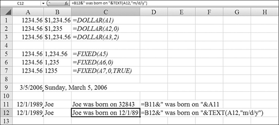
Today, the TEXT function is the most versatile solution to this problem. If you understand the basics of custom numeric formatting codes, you can easily use TEXT to format a date or a number in any conceivable format. For example, the formula in Cell C12 uses =TEXT(A12,"m/d/y") to force the date to display as a date.
The TEXT function gives you a lot of versatility. To learn the custom formatting codes for a cell, you can select the cell, display the Format Cells dialog (by pressing Ctrl+1), and choose the Custom category on the Number tab. Excel shows you the codes used to create that format.
If you don’t care to learn the number formatting codes, you can use either the DOLLAR or FIXED function to return a number as text, with a few choices regarding number of decimals and whether Excel should use the thousands separator. The formulas shown in C2:C7 in Figure 23.58 return the formatted text values shown in Column B.
Syntax: =TEXT(value,format_text)
The TEXT function converts a value to text in a specific number format. Formatting a cell with an option on the Number tab of the Format Cells dialog changes only the format, not the value. Using the TEXT function converts a value to formatted text, and the result is no longer calculated as a number.
The TEXT function takes the following arguments:
value—This is a numeric value, a formula that evaluates to a numeric value, or a reference to a cell that contains a numeric value.format_text—This is a number format in text form from the Category box on the Number tab in the Format Cells dialog box.format_textcannot contain an asterisk (*) and cannot be the general number format.
Syntax: =DOLLAR(number,decimals)
The DOLLAR function converts a number to text using currency format, with the decimals rounded to the specified place. The format used is $#,##0.00_);($#,##0.00). The major difference between formatting a cell that contains a number with the Format Cells dialog and formatting a number directly with the DOLLAR function is that DOLLAR converts its result to text. A number formatted with the Cells command is still a number. You can continue to use numbers formatted with DOLLAR in formulas because Microsoft Excel converts numbers entered as text values to numbers when it calculates.
The DOLLAR function takes the following arguments:
number—This is a number, a reference to a cell that contains a number, or a formula that evaluates to a number.decimals—This is the number of digits to the right of the decimal point. Ifdecimalsis negative,numberis rounded to the left of the decimal point. If you omitdecimals, it is assumed to be2.
Syntax: =FIXED(number,decimals,no_commas)
The FIXED function rounds a number to the specified number of decimals, formats the number in decimal format using a period and commas, and returns the result as text. The major difference between formatting a cell that contains a number with the Format Cells dialog and formatting a number directly with the FIXED function is that FIXED converts its result to text. A number formatted with the Format Cells dialog is still a number. This function takes the following arguments:
number—This is the number you want to round and convert to text.decimals—This is the number of digits to the right of the decimal point. Numbers in Microsoft Excel can never have more than 15 significant digits, butdecimalscan be as large as 127. Ifdecimalsis negative,numberis rounded to the left of the decimal point. If you omitdecimals, it is assumed to be2.no_commas—This is a logical value that, ifTRUE, preventsFIXEDfrom including commas in the returned text. Ifno_commasisFALSEor omitted, the returned text includes commas as usual.
Using the T and VALUE Functions
The T and VALUE functions are left over from Lotus days.
=T("text") returns the original text. If Cell B1 contains the number 123, =T(B1) would return an empty text. Basically, T() returns the value in the cell only if it is text.
=VALUE() converts text that looks like a number or a date to the number or the date.
Using Functions for Non-English Character Sets
There are 11 more functions that have not been covered in this section. These functions deal with text in character systems where each character takes up more than 1 byte. This is true in many Asian languages. The following functions are beyond the scope of this edition: ASC, BAHTTEXT, FINDB, JIS, LEFTB, MIDB, PHONETIC, REPLACEB, RIGHTB, SEARCHB, YEN but are described earlier in this chapter, in Table 23.3.
Excel Troubleshooting: Text Times Entered as M:SS Instead of H:MM:SS
In Figure 23.59, Column B contains a series of time trial results. When you total the column in Cell B12, you realize that all the times were entered as text.
Figure 23.59. You can use the LEFT and RIGHT text functions to provide the arguments for the TIME function.

The formulas in Column C use =TIMEVALUE(B2). However, a time such as 2 minutes 50 seconds is converted in the function to 2 hours 50 minutes. In this case, TIMEVALUE does not work.
There are two alternative strategies:
- One solution is to use the
TIMEfunction. In Column D, the text times are converted to real times by using theTIMEfunction. In each case, the hours should be zero. The minutes are=LEFT(B2,1). The seconds are=RIGHT(B2,0). The formula in Cell D2 is=TIME(0,LEFT(B2,1),RIGHT(B2,2)). You copy this formula down and format the range as a time. - The other solution is to use the concatenation operator to pad the left of Column B with
0:0. This allows the text to work in theTIMEVALUEfunction. The formula in Cell E2 is=TIMEVALUE("0:0"&B2). Again, you need to copy this formula down and format the range as a time.