Chapter 8. Fabulous Table Intelligence

In this chapter

Defining Suitable Data for Excel Tables 132

Keeping Headers in View 133

Adding a Total Row to a Table 137

Toggling Totals 138

Expanding a Table 138

Adding New Formulas to Tables 139

Selecting Only the Data in the Column 142

Using Table Data for Charts to Ensure Stickiness 145

Replacing Named Ranges with Table References 146

Creating Banded Rows and Columns with Table Styles 149

Dealing with the AutoFilter Drop-Downs 152

A fundamental use of Excel is for analyzing two-dimensional tables of data. Most worksheets contain headings at the top and then rows of data. Most Excel customers spend a lot of time working with tables of data. Microsoft recognized this and added intelligent tables to Excel 2007. If you explicitly tell Excel 2007 that you are working on a table of data, it displays a custom Table ribbon that has a number of amazing features.

Some of the benefits of Excel’s intelligent tables include the following:

• You can automatically add AutoFilter drop-downs to the headings in a table.
• You have one-click access to banded rows, banded columns, and other autoformats.
• You can toggle a total row on or off.
• You have one-click access to removing duplicates.
• You can automatically copy new formulas to all cells in a column.
• You can automatically extend a table when new data is typed below or to the right of the table. This feature also affects any charts, formulas, or pivot tables that pointed to the table, causing them to expand as well.
• You can extend conditional formatting to new rows in the table.
• You can automatically freeze panes to show the heading row as you scroll off the page.
• You can automatically set up range names for an entire table and each column within the table.

Defining Suitable Data for Excel Tables

Many Excel spreadsheets contain data that is not suitable for Excel tables. For the purpose of this chapter, a table is a range of Excel data. Each row in the range is one record of data. Each row might describe, for example, an invoice or a customer or an inventory item. Each column in the table creates another field for each row. Fields might include invoice number, customer name, total sales, and so on. A table usually has headings in the first row.

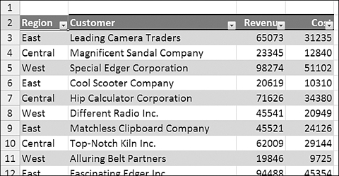
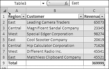
The simple range in Figure 8.1 would make a suitable table because each row in this range is a record, and each column is a field.

Figure 8.1. This would make an ideal table in Excel.

Defining a Table

There are four ways to create a table in Excel 2007:

• Select a cell in the dataset and choose Insert, Tables, Table.
• Select a cell in the dataset and choose Home, Style, Format as Table. Choose a Style and then press OK.
• Select a cell in the dataset and press Ctrl+T.
• Select a cell in the dataset and press Ctrl+L. (In Excel 2003, tables were originally called lists. Ctrl+L was the shortcut for a list.)

When you use any of these methods, Excel uses IntelliSense to determine the edge of the table. Excel looks for a completely blank row and a completely blank column to define the edges of the table.

Excel shows the suspected table range in the Create Table dialog, as shown in Figure 8.2. You need to verify that this range is correct. If your table has headers, you leave the My Table Has Headers check box checked and press OK.

Figure 8.2. Excel’s IntelliSense guesses the extent of the table.

As shown in Figure 8.3, Excel adds a default table format to your range. The headings gain autofilter drop-downs. A new ribbon called Table Tools—Design is displayed. Excel assigns a name similar to Table1 to the table. Don’t worry; if any of this is annoying to you, you can turn off many of the features with a click of the mouse.

Figure 8.3. The table has an interesting autoformat, but there are many more features.

Keeping Headers in View

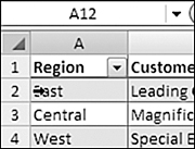
Notice that in Figure 8.3, the headings appear in Row 2 of the worksheet. As you scroll down through the table, you can eventually scroll to the point where Row 2 is no longer visible in the window. At this point, Excel moves the headings from Row 2 and shows them where column names A, B, C, D normally display. Figure 8.4 shows the headings as column names.

Figure 8.4. When you do not use the Freeze Panes command, Excel automatically moves the heading values up to the column names when you scroll the headings off the window.

These heading names stay as column names as long as all these are true:

• The cell pointer is inside the range of the table.
• The header row is not visible in the window.
• At least one row of the table is visible in the window. If you leave the cell pointer in the table and then use a scrollbar to scroll the table out of view, the column names revert to column letters.

Once any of the above conditions is no longer true, the headings disappear from the column name area.

Freezing Worksheet Panes

Excel 2007’s automatic heading visibility feature is very cool. With earlier versions of Excel, many did not know there was a way to freeze panes. Whether you knew about that feature or not, it is a positive feature 90% of the time, though it’s not perfect.

One problem with Excel 2007’s automatic heading visibility feature is that the autofilter drop-downs disappear from the headings when they are scrolled up to the column names.

Second, it is a bit annoying that the headings disappear when you select a cell outside the table. I think that if I can see part of a table in the window, Excel should keep the headings up as part of the column names. The cell pointer can be a distraction in a dataset, and if, for example, you are showing your manager something on the screen, you might have a tendency to click outside the table so that the manager does not think you are trying to show him one particular cell.

Third, the automatic heading visibility feature does not work for the first column. In Figure 8.5, for example, a wide table has labels in Column A. After you choose First Column, Excel properly formats Column A. However, if you scroll over to see the month of December, Excel does not make the Column A values stay visible.

Figure 8.5. The automatic heading visibility feature doesn’t work for the first column.

The old-style Freeze Panes command is still available and is even a bit easier to use in Excel 2007.

In prior versions of Excel, you were forced to put the cell pointer in the first cell that should not be frozen before invoking the Freeze Panes command. In Excel 2007, Microsoft has added two new commands that allow you to freeze the first row or the first column from anywhere. Here’s how you freeze the first row:

1. Make sure the row that you want to stay at the top of the window is the first visible row in the window.
2. From the Window group of the View ribbon, select Freeze Panes. The drop-down that appears is shown in Figure 8.6.

   Figure 8.6. Excel 2007 adds two new commands to the Freeze Panes area.

   

3. Select Freeze Top Row.

You can now scroll anywhere on the worksheet and always see the first row.

It is annoying, but the Freeze First Column resets the Freeze First Row icon, and vice versa. If you need to freeze both the first column and first row, you will have to use the Freeze Panes command as described in the following sections.

Clearing Freeze Panes

To turn off the Freeze Panes option, you again select the Freeze Panes icon in the View ribbon. The first option in the drop-down is now Unfreeze Panes. You can select this option to unlock the view; you can then scroll anywhere in the window.

Using the Old Version of Freeze Panes for Absolute Control

There may be times when you want several rows or columns to remain visible. Just as in previous versions of Excel, you can do this when you understand how Freeze Panes works.

Consider the worksheet in Figure 8.7. You would always want to see the data in Columns A:D at the left side of the window. There are several rows of title information that don’t necessarily need to be visible at the top of the worksheet as you scroll, but it would be good to see Rows 5 and 6 at the top of the window as you scroll.

Figure 8.7. This worksheet is too complex for the new Freeze Top Row command to actually work as desired.

You can set up the headings to stay visible by following these steps:

1. Click the arrow at the bottom of the vertical scrollbar four times to make Row 5 the first row visible in the window.
2. Select the first cell that will not be frozen in the window. Everything visible in the window above and to the left of this cell will be frozen. In Figure 8.8, this would be Cell E7. It is critical that you select this cell before moving on to step 3.

   Figure 8.8. You select the first cell that won’t be frozen.

   

3. From the Window group of the View ribbon, select the Freeze Panes dropdown. Then select Freeze Panes again.

The result is that you can scroll down and right. Even out at Column V, Row 62, you can see the headings in Rows 5:6 and the values in Columns A:D, as shown in Figure 8.9.

Figure 8.9. After you use the original Freeze Panes command, you can have multiple rows and columns frozen at the top and left of the worksheet.

The key to using the Freeze Panes command is that you must place the cell pointer before using the command. The command freezes everything that was above and to the left of the cell pointer location when the command was invoked.

To freeze only Columns A:B and no rows, you would invoke the command from Row 1 of Column C. Because there is nothing above the cell pointer, no rows are frozen.

Adding a Total Row to a Table

There is a Totals Row checkbox in the Table Styles Options group of the Table Tools Design ribbon. When you select this box, Excel automatically adds a total to the bottom of your table.

By default, Excel adds the word Total to the first column of the table and adds a formula to the right-most column of the table to sum the column.

Figure 8.10 shows the default total row for a table. To add a sum formula to Column C, you select the cell for Column C in the total row. When a drop-down arrow appears, you select Sum from the list.

Figure 8.10. Clicking the Total Row check box in the ribbon adds a default total row. You use the drop-downs to change the function or add totals to other columns.

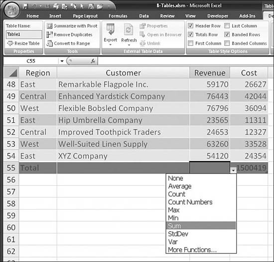
In Figure 8.10, instead of using the SUM formula, Excel uses the SUBTOTAL function, with a first argument of 109. The SUBTOTAL function is similar to the SUM function, with two exceptions. First, the function ignores other SUBTOTAL functions in the range. Second, with a first argument in the 101–109 range, Excel ignores any values that are hidden, including rows that are hidden by the autofilter drop-downs.

The total cost in Figure 8.10 is $1.4 million. In Figure 8.11, the Region column is filtered to only the Central region. Because the SUBTOTAL function ignores hidden rows, the total cost automatically updates to show $448,511.

Figure 8.11. You choose a region from the autofilter drop-down, and the SUBTOTALS function reflects the total of the visible rows.

Toggling Totals

When you use tables, you can toggle the total row on and off. You use the Total Row check box in the Table Tools Design ribbon to turn on or off the totals. In most cases, Excel remembers when you have customized the totals to provide totals for the last two columns. However, you might find that if you add new columns to a table, you will have to add these totals to the new columns using the dropdown in the total row.

Expanding a Table

A common feature of tables is that they tend to grow and expand. Every day, you might add new records to a table or paste new records to the bottom of a table. Or, you might add a new column with a new calculation.

Excel can automatically expand a table, or you can choose to expand a table manually. When you expand a table, any references to the table automatically expand.

Adding Rows to a Table Automatically

The easiest way to add rows to a table is from the last row of the table. If you are in the last column of the last row and press the Tab key, Excel adds a new row to the table and moves the cell pointer to the first column in the new row. This behavior is similar to existing functionality in tables in Microsoft Word.

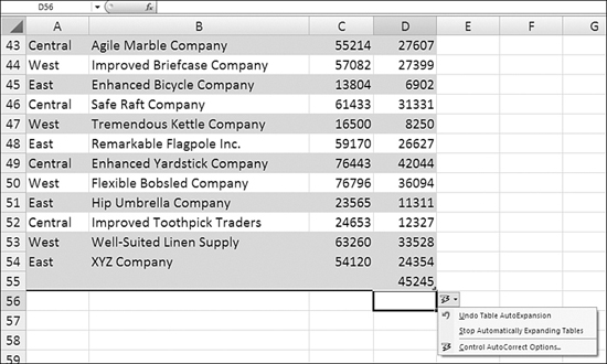
However, the simplest way to add a new row to a table is to click in the blank row under the table and type new data. As soon as you enter something in a cell just below the table, Excel expands the table formatting to include the new row. Excel also displays an AutoCorrect lightning bolt icon. If you don’t want Excel to automatically expand the table, you can use the drop-down next to this icon to undo the table AutoExpansion, as shown in Figure 8.12.

Figure 8.12. If you type a new value below the table, Excel automatically extends the table to include the new row.

Manually Resizing a Table

The bottom-right cell of a table contains a small angle-bracket in the lower-right corner of the cell. You can use this angle-bracket to manually extend the table.

When you click the angle-bracket, you can either drag down to add more rows or drag right to add more columns to the table.

You can also select Table Tools, Design, Properties, Resize Table. The Resize Table dialog appears, allowing you to specify the new range for the table. There are a few limitations. For example, you cannot change the header row during this process.

Adding New Columns to a Table

To add a new column to a table, you go to the blank cell to the right of the last header and type a new header for the column. Excel automatically extends the table by another column and copies any table formatting to the new column. The AutoCorrect lightning bolt icon appears. If you don’t want the new column to be part of the table, you use the drop-down next to the AutoCorrect icon to undo the table AutoExpansion.

Adding New Formulas to Tables

Way back in Excel 97, Microsoft added something called Natural Language Formulas to Excel. With Excel 2007, those old formulas are officially depreciated. However, the new-style table formulas are reminiscent of those formulas.

In Figure 8.13, a new column has been added to the table, with the heading Profit. To add a formula to that column, you follow these steps.

1. Select Cell E3.
2. Type an equals sign.
3. Using either the mouse or the arrow keys, select the first revenue cell in C3. Note that the formula is unlike any formula that you’ve seen before. It starts out with =[Revenue], as shown in Figure 8.13.

   Figure 8.13. When you start entering a formula in a table, Excel uses table nomenclature for the formula references.

   

4. Type a minus sign.
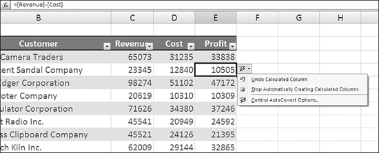
5. Click Cell D3 for Cost. The formula now reads =[Revenue]-[Cost], as shown in Figure 8.14.

   Figure 8.14. Without adding any named ranges, the formula =[Revenue]-[Cost] is easier to understand than D3–C3.

   

6. An amazing thing happens when you press the Enter key to accept the formula: Excel automatically copies the formula down to all rows in the table, as shown in Figure 8.15.

Figure 8.15. The new formula is automatically copied to all rows of the table.

In prior versions of Excel, after adding a formula to a new column, you had to double-click the fill handle to copy the formula down to all rows of the table. This new functionality will save you time.

If you don’t want to have the formula copied down to all rows, you can undo the behavior by selecting the AutoCorrect icon and then choosing the appropriate option.

Stopping the Automatic Copying of Formulas

You might at some point have a column in a table and not want Excel to use the same formula everywhere in the column. Excel 2007 calls this a calculated column exception. Because any formula that you enter in the column is automatically copied to the entire column, you need to use special care to set up a calculated column exception.

Say that you already have a formula in a column and want to change to a different formula in just one cell. In this case, you follow these steps:

1. Enter the different formula in the one cell. Excel automatically copies the formula to the entire column.
2. Immediately click the Undo button in the Quick Access toolbar.

Excel marks this cell with a green triangle. If you hover your mouse over the green triangle, Excel tells you, “This cell is inconsistent with the column formula.”

There are other ways to set up a first column exception:

• Type data other than a formula in a calculated column cell.
• Delete a single formula from one or more cells in the calculated column.
• Move or delete a cell on another worksheet area that is referenced by one of the rows in the calculated column. This basically changes the formula in that one cell, creating a column exception. Excel then stops copying the calculation in that column.

Formatting the Results of a New Formula

The automatic copying of formulas includes one minor annoyance. In prior versions of Excel, you would add a new column by following these steps:

1. Type the heading.
2. Type the first formula.
3. Format the first formula.
4. Double-click the fill handle to copy the formula.

Now that Excel is, in essence, performing the last step for you, there is no chance to format the first cell before it gets copied. In Figure 8.16, the calculation for gross profit percentage was copied before the cell could be formatted as a percentage.

Figure 8.16. Excel copies a formula down to all rows before you have a chance to format the new column.

You can try formatting Cell F3 before entering the formula, but the table logic appears to overwrite this format when the formula is copied to the column. Thus, you have two options:

• Format the top cell as a percentage and then double-click the fill handle to copy the formatted cell down to all rows of the table.
• Select the table column first and then apply the percentage format to the entire column.

Selecting Only the Data in the Column

There are several new options you can use when selecting data in a table. If you are going to format a table, you probably just want to format the numbers in the table and not the headings. Excel has added distinct methods for selecting the data portion of a column or selecting the entire table column with headings and totals.

Selecting by Right-Clicking

One way to select the data in a column is to right-click on a cell in the table. From the context menu, you choose the Select option. The flyout menu offers three choices, as shown in Figure 8.17:

• Table Column Data—You select this option to select just the data rows of that column. This skips the heading row and the total row.
• Entire Table Column—You select this option to include the heading for the column and the cell in the total row.
• Table Row—You select this option to select an entire row of a table.

Figure 8.17. You can right-click to select the data in the column.

Selecting by Using Shortcuts

You can also use the old Excel shortcuts to select rows or columns. These shortcut keys are modified when you are in a table:

• You can press Shift+Spacebar once to select an entire row in a table.
• You can press Shift+Spacebar a second time to select the entire worksheet row.
• You can press Ctrl+Spacebar once to select the table data in the current column of the table. This excludes the total row and the heading row. Figure 8.18 shows the selection after pressing Ctrl+Spacebar once from Cell C6.

Figure 8.18. You can press Ctrl+Spacebar once to select the data portion of the current column.

• You can press Ctrl+Spacebar again to expand the selection to include the heading and total cell for that column, as shown in Figure 8.19.

Figure 8.19. You can press Ctrl+Spacebar a second time to expand the selection to include the heading and total cells.

• You can press Ctrl+Spacebar a third time to select the entire worksheet column.

Selecting by Using the New Arrow Mouse Pointers

Excel has added a new arrow mouse pointer that you can use in selecting table rows and table columns. The use of this mouse pointer is a bit tricky. The following figures show some examples:

• In Figure 8.20, the mouse is hovering over the lower half of the Column A column letter. In this position, Column A is highlighted. You can click here any number of times to select the entire column.

Figure 8.20. The traditional select column mouse pointer causes the row letter to be highlighted.

• In Figure 8.21, the mouse is hovering over the top half of Cell A1. This is the first row of the table. The first click here selects A2:A8. The second click here selects A1:A9. Alternating clicks toggle between A2:A8 (the table data without headers and totals) and A1:A9 (the complete table column).

Figure 8.21. You can move just a bit into the table header, and the new (but identically appearing) mouse pointer takes over.

• In Figure 8.22, the mouse is hovering over the top-left corner of Cell A1. The first click here selects A2:C8 (the table without headings and totals). The next click selects A1:A9 (the entire table). Additional clicks toggle between these two selections.

Figure 8.22. You can move to the corner of the table to get the new table selection mouse pointer.

• In Figure 8.23, the mouse is hovering near the left edge of Cell A2. Clicking here any number of times selects the entire table row (that is, A2:C2).

Figure 8.23. At the left edge of a table row, the new table row selection pointer appears.

If you are a heavy-duty user of Excel, you will likely find yourself using these new table selection methods. The new conditional formatting options such as data bars and color scales require you to select the data in a column without the total row. Mastering the various selection methods will greatly enhance your ability to work with the new formatting.

Using Table Data for Charts to Ensure Stickiness

When you define a range as a table and expand the table, any references to the table also expand. If you routinely have to re-create new charts every month when you receive new data, you will love this feature.

Before creating a chart, you make a table out of the underlying data. In Figure 8.24, for example, the chart is based on the table in A1:D4. Currently, the chart has three months’ worth of data.

Figure 8.24. This chart is based on the table in A1:D4.

If you type a heading for the new month in Cell E1, immediately, the chart redraws to include data for April. You fill in the data for the new month, and you will not have to ever re-create a chart; the new data is added to the chart, preserving the old formatting, as shown in Figure 8.25.

Figure 8.25. You add new data to the table, and the chart automatically expands.

Replacing Named Ranges with Table References

A benefit of using tables is that Excel understands a new reference style for formulas that point to data in a table. A new name is created automatically when a table is defined. The name includes the name of the table (something like Table1) and the name of the column.

The biggest benefit of this new referencing style is that the ranges that the names refer to are expanded automatically when the table expands. This new referencing style will eliminate many of the chances for error that existed with using named ranges.

Referencing an Entire Table from Outside the Table

When a table is defined, it becomes easier to reference the table from outside the table. Figure 8.26 shows a sales rep lookup table. Because this is the first table in the workbook, Excel has assigned the name Table1 to this table.

Figure 8.26. This sales rep lookup table is automatically assigned the name Table1.

Figure 8.27 shows an invoice register located on another sheet in the workbook. Like many mainframe reports, this one includes the sales rep number, without the name and region information. To add a VLOOKUP function to Figure 8.27 that references Table1, follow these steps:

1. Start to type a VLOOKUP formula in Column D. When you get to the second argument, type the letter T, and the AutoComplete list scrolls down to the T entries. Among the function names are entries for Table1 and Table2, as shown in Figure 8.27.

   Figure 8.27. Even though there are no defined names in the workbook, Excel understands the Table1 nomenclature.

   

2. Select Table1 from the list and press Tab.
3. Finish the formula so that it is =VLOOKUP($B2,Table1,COLUMN(B2),False).
4. Copy the formula to the rest of the range. Like chart references, table references are sticky. In Figure 8.28, there are a couple records for a new sales rep, S26. This rep is not yet in the original table.

   Figure 8.28. When you add the missing reps to Table1, the references here to Table1 expand as well.

   

5. Go back to the original table and add a new row with S25 data. All the formulas that reference Table1 automatically recalculate to include the new rows.

Referencing Table Columns from Outside a Table

To reference an entire column from outside a table, you use the syntax TableName[ColumnName]. When you do this, Excel’s AutoComplete feature provides a list of column names for you. After you type Table1[, the AutoComplete list shows all the columns in the table, plus additional keywords (which are discussed in the following section, “Using Structured References to Refer to Tables in Formulas”). The AutoComplete list is shown in Figure 8.29.

Figure 8.29. Excel offers AutoComplete entries from which you can choose the column name when entering a formula.

References to a table column do not include the header or total row. While this behavior is usually desired, there might be instances when you use a INDEX or OFFSET function that you expect Excel to include the heading as row 1 in the function.

The formula in Figure 8.30 uses three references to a table to find the sales for a particular product and a particular region. The nomenclature Quantity, Product, and Region is easier to understand than cell addresses such as D2:D87. This is the complete formula in Cell G3:

=SUMIFS(Table1[Quantity],Table1[Product],$F3,Table1[Region],G$2)

Figure 8.30. This formula is a fairly complex conditional sum. It relies on three columns from the table.

Table references are valid on any worksheet in the workbook. If you want to refer to a table that is seven worksheets away, you can still use the Table1 nomenclature, without prefixing the worksheet name.

Using Structured References to Refer to Tables in Formulas

Microsoft has created a fairly comprehensive way to refer to various parts of tables. You’ve seen some of the table nomenclature syntax in the previous two sections. The following are complete details for writing formulas that refer to tables:

• The reference to a table starts with the table name. If you are creating the formula within the table itself, you can omit the table name.
• If no further qualifiers are entered, the table name refers to the data rows of the table. This excludes the headings and total rows.
• Further qualifiers should be enclosed in square brackets. If you are using one qualifier, only one set of square brackets is needed. You may specify TableName[Qualifier] or TableName[[Qualifier]].
• If you are specifying multiple qualifiers, each qualifier must be surrounded by square brackets. The qualifiers must be separated by commas. The complete set of qualifiers must be surrounded by square brackets. The syntax follows this pattern: TableName[[Qualifier1],[Qualifier2],Qualifier3]].
• For a table with a header row, each column heading is automatically added to the list of qualifiers.
• For a table without a header row, the list of qualifiers includes Column1, Column2, and so on.
• Every table also has these qualifiers: #All, #Data, #Headers, #Totals, #ThisRow.
• The #ThisRow qualifier must be used in conjunction with another qualifier.

This system allows you to select a wide variety of references without having to use cell references. To get the total of sales from Table1, you can either use =SUM(Table1[Sales]) or =Table1[[#Total],[Sales]]. The second syntax returns a #REF! error if someone turns off the Totals Row check box in the Table Tools Design ribbon.

Figure 8.31 shows various structured references.

Figure 8.31. Structured references are shown in Column I.

Creating Banded Rows and Columns with Table Styles

In previous versions of Excel, creating banded rows or columns required creative conditional formatting or tedious manual work. Creating banded rows or columns in a table is relatively simple in Excel 2007.

The fourth group on the Table Tools Design ribbon is Table Style Options. This group includes check boxes for Banded Rows and Banded Columns. These check boxes work only if the selected table style includes rules for banded columns and/or banded rows. If you have selected the plain white table style, turning on or off banded rows and columns will have no effect.

Figure 8.32 shows five tables. The first table contains banded rows. The second table has banded columns. The third table leaves banded rows and columns off, but the first column, last column, header row, and total row are checked. The top table in Column H contains both banded rows and banded columns. The last table contains a custom format to change the banding from one stripe to two stripes. The next section provides details on how to customize the table style.

Figure 8.32. These tables exhibit various combinations of the table style options. The fifth table requires a customization of the table style.

Customizing a Table Style: Creating Double-Height Banded Rows

At the bottom of the Table Styles gallery, there is a New Table Style button. I would encourage you not to use this button! It can be rather intimidating to set up a completely new style. It is often easier to start with an existing style and modify it. To do this, you right-click a style and choose Duplicate, as shown in Figure 8.33.

Figure 8.33. Rather than choosing New Table Quick Style, you can choose to duplicate an existing style.

After you choose Duplicate, Excel displays the Modify Table Quick Style dialog box. Excel assigns a new name to the style, adding a 2 to the existing style name. You can rename the style if you like.

To create double-height banded rows, you follow these steps:

1. Choose First Row Stripe from the Table Element list. A Stripe Size drop-down appears.
2. Choose 2 from the Stripe Size drop-down.
3. Choose Second Row Stripe from the Table Element list. A Stripe Size drop-down appears.
4. Choose 2 from the Stripe Size drop-down.
5. If you would like your modified theme to be the default style for all new tables created in this document, choose the Set as Default Table Quick Style for This Document check box in the lower-left corner of the dialog.

   Figure 8.34. For double-height row banding, you change the stripe size.

   

6. Click OK, and your custom style is saved to a new Custom section at the top of the Table Styles drop-down.

Creating Banded Rows Outside a Table

You might find some of the table behavior annoying. If you want banded columns but don’t want to use a full-fledged table, you can temporarily create a table, apply a banded row format to the table, and then convert it back to a range in order to have a banded row format on the range. Here’s how you do it:

1. Select a cell in the range to be formatted.
2. Press Ctrl+T to make the range a table.
3. If your default table style does not include banded rows, choose a new table style from the Table Styles gallery on the Table Tools Design ribbon.
4. In the Table Tools Design ribbon, choose Tools, Convert to Range. This removes the table properties but keeps the table formatting.

Dealing with the AutoFilter Drop-Downs

A common spreadsheet style rule says that you should right-justify the headings above numeric columns. If you regularly follow this convention, you will certainly be annoyed with the default choice that all tables are automatically created with the autofilter drop-downs applied.

In Figure 8.35, the first range contains data with the Q1 headings in the first row. If you apply a table to a range, the autofilter drop-downs completely cover the headings, making the table useless. The table in Rows 10:16 shows this.

Figure 8.35. The headings in Row 1 become unusable when the range is converted to a table.

One option, shown in Row 19, is to begin centering your headings instead of right-justifying them.

The final option, shown in Row 27, is to keep the table but turn off the autofilter for the table. Frustratingly, this option does not appear on the Table Tools Design ribbon. Instead, you need to go to Home, Editing, Sort & Filter, Filter to toggle away the drop-downs.

There are more tricks available for tables. See Chapter 13, “Removing Duplicates and Filtering,” and Chapter 14, “Sorting,” for more table tricks.