Chapter 13. Removing Duplicates and Filtering

In this chapter

Using Remove Duplicates to Find Unique Values 272

Filtering Records 275

Using the Advanced Filter Command 284

Duplicate data is a common problem in Excel. Microsoft has provided new tools in Excel 2007 to make finding and eliminating duplicates easier.

Autofiltering has been in Excel for a decade, but it has received a makeover in Excel 2007. The autofilter drop-downs now allow you to multiselect values and offer new smart filters.

The Advanced Filter command continues to be available, still as complicated as ever. The hope is that with the excellent improvements to autofiltering and the addition of duplicate handling, you will never have to turn to Advanced Filter. In previous versions of Excel, I almost always had to resort to using Advanced Filter to find a list of unique values. The new Remove Duplicates command allows you to find unique values with a couple mouse clicks.

Using Remove Duplicates to Find Unique Values

By its nature, transactional data has a lot of detail. You end up with transactional data in Excel because it is often the easiest to obtain. As you start to analyze transactional data, you often want to find the number of customers or number of products or number of something in the dataset.

Transactional data can tell you, for example, that there were 34 invoices issued last month, but that doesn’t mean there were 34 customers. Some of those customers might have bought from you repeatedly, so that 20 customers could account for 34 invoices. To find the number of unique customers, you need to find a way to eliminate the duplicate records in a dataset. In the past, this usually meant using Advanced Filter or possibly a pivot table. In Excel 2007, there is a new data tool to remove duplicates, called Remove Duplicates, and it is much easier to use.

The first thing to realize is that the Remove Duplicates tool is destructive. It really removes the duplicate records. If you want to keep the original transactional data intact, you should make a copy of the customer column in a blank section of the workbook (or make a backup copy of the workbook).

To find the unique values in a dataset, you follow these steps:

1. Copy the dataset to a blank section of the worksheet. Make sure to leave a blank column between your real data and the copy of the data.
2. Select a single cell within the dataset.
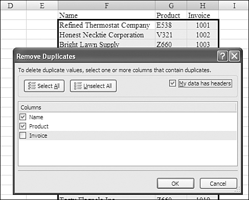
3. On the Data ribbon, in the Data Tools group, choose Remove Duplicates. Excel expands the selection to include the entire range. In the Remove Duplicates dialog, Excel predicts whether your data has headers. This dialog also shows a list of the fields in the dataset. In Figure 13.1, for example, the goal is to find a unique list of customers.

   Figure 13.1. You choose which columns should be considered when analyzing duplicates.

   

4. You don’t care about the invoice numbers, so uncheck Invoice from the Columns list.
5. Click OK to perform the action. Excel tells you how many duplicate values were found and removed, and it also tells you how many unique values remain.

Removing Duplicates Based on Several Columns

In the previous set of steps, you analyzed only a single column when looking for duplicates. Sometimes, you need to find each unique combination of two fields (for example, a list of each unique combination of customer and product).

In this case, you follow these steps:

1. Copy the dataset to a blank section of the worksheet. Make sure to leave a blank column between your real data and the copy of the data.
2. Select a single cell within the dataset.
3. On the Data ribbon, in the Data Tools group, choose Remove Duplicates.
4. In the Remove Duplicates dialog, leave the boxes for both the Name and Product columns checked, as shown in Figure 13.2.

Figure 13.2. To find each unique combination of customer and product, you choose both fields.

In this case, the result is a list of all products ordered by each customer.

Handling Duplicates Other Ways

The Remove Duplicates command is also available in Table Tools, Design ribbon. If you have defined a table as a range, you can remove duplicates from that ribbon.

Remember that the Remove Duplicates command is destructive. Sometimes, you might want to find the duplicates and choose which version to remove. In that case, you choose Home, Conditional Formatting, Highlight Cell Rules, Duplicate Values.

→  To learn more about choosing which duplicates to remove, see “Identifying Duplicate or Unique Values Using Conditional Formatting,” page 173, in Chapter 9.

Other times, you might want to send a copy of the unique values to a new location. In that case, you use the Advanced Filter command discussed later in this chapter.

Finally, you might want to remove duplicates but add up the sales for all the removed records and add them to the Customer field. While this can be achieved with pivot tables, it can also be achieved by using the Consolidate feature, which is discussed in the next section.

Combining Duplicates and Adding Values

In Figure 13.3, each customer appears one or more times in the list with a sales value. In addition to finding a unique list of customers, you would like to know the total sales for each customer.

Figure 13.3. You start at a blank section of the workbook before invoking the Consolidate feature.

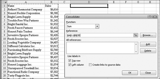
Although you could use a pivot table to find the total sales for each customer, you can also use the data tools to consolidate the table down to one record per customer, with the total sales from all the records for that customer. Here’s how you do it:

1. Do not pre-select the data. Instead, move the cell pointer to a blank section of the worksheet.
2. Select Data, Data Tools, Consolidate. The Consolidate dialog box appears.
3. In the Consolidate dialog box, enter the reference to your data in the Reference box. The data will be combined based on the field in the left column of the range. If you had multiple lists of customers, you could click the Add button and enter additional ranges.
4. Make sure to check the Top Row and Left Column check boxes in the Use Labels in section.
5. Click OK.

Excel creates a new table. Each customer appears in the table just once. The sales associated with all the records of the customer appear in the new total, as shown in Figure 13.4.

Figure 13.4. The total sales in Columns B and E are the same.

Two annoyances remain with this command. First, the heading for the leftmost column is never filled in. Second, the command leaves the results in the same sequence in which they originally appeared. In this example, you will probably want to add the heading to Cell D2 and also sort the data.

Filtering Records

Microsoft added powerful new features to the Filter command in Excel 2007. (This feature was formerly called AutoFilter, but it has been renamed simply as a Filter in Excel 2007.) Filtering works on any range of data with headings in the first row of the range. It works with ranges that have been defined as tables as well as regular ranges.

The following are some new features in Excel 2007 filtering:

• Multiselection is available in the filter drop-down. If you want to select rows that meet one of two values or rows for all but one particular value, this is now possible, using the regular filter.
• You can filter by color or icon set.
• You can filter text columns based on cells that begin with a value, end with a value, or contain a value.
• You can filter number columns based on cells that are greater than, less than, or between values. You can choose Top 10, Above Average, or Below Average.
• You can filter date values by year or month. You can filter to conceptual values such as this month, last quarter, or year to date.
• You can filter by selection. Rather than choosing from the filter drop-down, you can right-click any value and choose to filter based on the selected cell’s value, color, font color, or icon.

The various features work great when one column contains values of the same type. For example, Excel expects that if you have dates in a column, all the cells except the header will be dates. Excel offers special text, number, or date formats based on what it sees in the column. These special formats are mutually exclusive: If you have a column with a mix of dates, numbers, and text, Excel offers only the special filtering type for the value type that occurs most frequently in the column. If you happen to have exactly 150 values with text, 150 values with numbers, and 150 values with dates, Excel offers the text filters. With a tie between dates and values, Excel offers the value filters.

Using a Filter

The icon to turn on the filter drop-downs toggles the feature on and off. To turn on the feature, you click the icon once. To turn off the feature, you click the icon again.

You need to select one cell in your data range before clicking the filter. You should have no blank rows or blank columns in the range to be filtered.

You can turn on the filter drop-downs by using any of these methods:

• From the Home ribbon, choose Editing, Sort & Filter, Filter.
• From the Data ribbon, choose Sort & Filter, Filter.
• Apply a table format to a range.
• Right-click any cell, choose Filter, and then select one of the options under Filter. In addition to performing the filter, this will turn on the filter feature if it was not previously turned on.

When the filter is turned on, a drop-down arrow is added to each heading in the range.

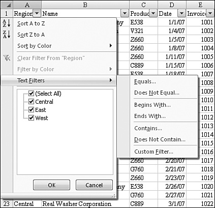
Figure 13.5 shows the menu available for one drop-down. This particular column includes text values, so the special filter flyout menu includes various special text filters.

Figure 13.5. The filter drop-down now features a multiselect list as well as new special filters.

Selecting One or Multiple Items from the Filter Drop-Down

In previous versions of Excel, the filter drop-down included a simple list of items in the column, and you would select one of the values. The multiselect nature of filters in 2007 offers far more power, but you have to exercise special care in using the drop-down.

Follow these steps to select a single item:

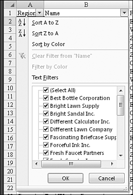
1. When you initially select the drop-down, all the items that appear in the column are selected with a check mark, as shown in Figure 13.6.

   Figure 13.6. By default, all the values in the column are selected.

   

2. To select a single value, first click Select All. This unchecks all the items in the list, as shown in Figure 13.7.

   Figure 13.7. Click Select All to remove the check mark from all items.

   

3. Click the value you want to filter on, as shown in Figure 13.8.

   Figure 13.8. When the checkmarks have been removed, you select the one value of interest and click OK.

   

4. Click OK at the bottom of the drop-down to apply the filter.

The process you use to filter to multiple values is similar. You first click Select All to remove the check marks from all items. You can then select the items that should be included in the filter.

The multiselection ability provides a vast improvement for filtering. You could argue that it now requires four clicks where the old autofilter required only two clicks, but the improvements are worth this hassle.

In the case where you need to select everything except one certain value, the new feature is set up perfectly. You select the drop-down, uncheck the undesired value, and click OK.

Identifying Which Columns Have Filters

Visual clues in Excel 2007 indicate that a filter has been applied to a dataset:

• The row numbers in the range appear in blue to indicate that the rows have a filter applied.
• The message area of the status bar in the lower-left corner of the screen shows a message similar to “22 of 34 records found.”
• The drop-down for the filtered column changes from a simple drop-down arrow to a Filter icon, as shown in Figure 13.9.

Figure 13.9. After you filter Column A to two values, the icon on the filter drop-down changes.

Combining Filters

Filters are additive. For example, if you place a filter on one column, you can then apply a filter to another column in order to show even fewer rows.

You cannot apply two filters to the same column. For example, you might want to select all the West region cells that are red. This is not allowed. Each column’s drop-down includes the list of values, a Filter by Color option, and a Special Filter option. From this complete list of filters for the one column, you can select only one filter.

Clearing Filters

After a filter has been applied, you have several options for clearing the filter:

• From the filter drop-down, select Clear Filter from Column. This leaves filters on in other columns.
• From the filter drop-down, choose a different filter.
• From the Data ribbon, choose Sort & Filter, Clear. This clears selected filters from any column but leaves the drop-downs in place so that you can continue to select other filters.
• Choose the Filter icon from the Data ribbon or the Home ribbon to clear all filters and turn off the filter feature.

Refreshing Filters

If data in a range changes, the filters do not automatically update. This could happen if you add new rows. It could happen if you edit data. It could also happen if your data range has formulas that point to lookup tables in other parts of the workbook.

In such a case, you need to have Excel calculate the filter again. Excel calls this feature Reapply. There are several ways you can reapply a filter:

• On the Data ribbon, select the Sort & Filter group and then click Reapply.
• On the Home ribbon, select Editing Group, Sort & Filter, Reapply.
• Right-click a cell and then choose Filter, Reapply.

Resizing the Filter Drop-Down

The filter drop-down always starts fairly small. If you have a long list of items, you might want the drop-down to be larger. To make this happen, you hover your mouse over the lower-right corner of the drop-down. When the mouse pointer changes to a two-headed diagonal arrow, you click and drag down or to the right.

Filtering by Selection

You can filter without using the filter drop-downs. Microsoft Access has offered a Filter by Selection icon in the toolbar for over a decade. Excel has finally added this functionality, but it is still hidden in an obscure place.

To access the feature, you right-click any cell and then choose Filter from the context menu. You then have an opportunity to filter based on the cell’s value, color, font color, or icon, as shown in Figure 13.10.

Figure 13.10. Although it is hidden, the Filter by Selection command provides a quick way to see all the other rows that match a single cell.

This feature works even if the filter drop-downs have not been activated previously. Using this feature turns on the filter drop-downs for the dataset.

It would be really cool if you could use this feature to multiselect values (for example, if you selected a cell that said East and then Ctrl+clicked on a cell for West). You might think that filtering by selection would filter to both East and West, but that does not work in Excel 2007. It would be excellent if Microsoft would add the ability to multiselect using this feature and would promote the feature to an icon on the ribbon in Excel 2009.

Filtering by Color or Icon

Cell colors are more prevalent in Excel 2007 than in prior versions, given the greatly improved conditional formatting tools. However, this feature also works with cells to which you have manually applied fill color.

Imagine that you are tracking numerous projects in Excel. You manually highlight certain projects in red if you are missing key elements of the project information. You can use Filter by Color to show only the rows that have red fill.

Filter by Color works for the cell color, the font color, or the icon in the cell. (Icons are available only from conditional formatting.)

→  For more information on icon sets, see “Setting Up an Icon Set,” on page 162, in Chapter 9.

As shown in Figure 13.11, the Filter by Color flyout menu offers to filter based on fill color, font color, or icon. Note that the sections of the flyout menu appear only if you have used color or icons in the range. If all your cells contain black text, Filter by Font Color will not appear in the flyout menu. If your range contains all black text on white background, without icons, the Filter by Color menu will be disabled.

Figure 13.11. The Filter by Color flyout menu offers to filter by icon, cell color, or font color.

Handling Date Filters

The default method for filtering a column of dates has changed dramatically in Excel 2007. In previous versions, the drop-down list contained a list of the dates in the column. In Excel 2007, Excel automatically groups the dates into hierarchical groups.

In Figure 13.12, the underlying data contains daily dates. However, the default drop-down shows options for the years found in the dataset.

Figure 13.12. Excel automatically groups dates up to years in the filter drop-down.

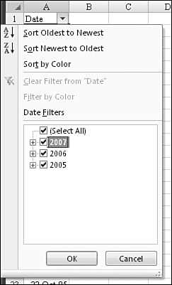
You click the plus sign next to any year to expand the list to show months within the year, as shown in Figure 13.13.

Figure 13.13. You can expand the hierarchical view to see months within the years.

You can then click the plus sign next to a month in order to see the days within the month.

Using Special Filters for Dates, Text, and Numbers

Excel examines the data in a column to determine whether it contains mostly text, mostly dates, or mostly numeric values. Depending on which data type appears most often, Excel offers special filters designed for that data type.

For columns that contain text, Excel has the filters Begins With, Ends With, Contains, Does Not Contain, Equals, and Does Not Equal. You are allowed to use wildcard characters in these filters. You can use an asterisk (*) for any number of characters or a question mark (?) to represent a single character.

For columns with numeric values, the special filters include Top 10, Above Average, Below Average, Between, Less Than, Greater Than, Does Not Equal, and Equals, as shown in Figure 13.14.

Figure 13.14. The special filters for numeric values give you the ability to find the above-average records or the top and bottom percentages, among other things.

For the filter named Top 10, you can specify the top or bottom values. You can specify whether the results are based on the top 10 items or the top 10% of items. Finally, you can change the number 10 to any number. Thus, you can use this filter to show the bottom 20% or the top 3 items.

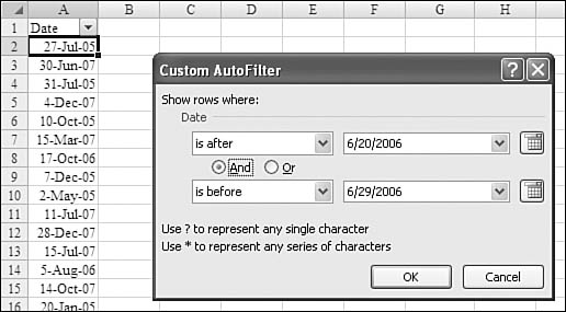
For columns with dates, the special filters include Before, After, or Between a particular day, week, month, quarter, or year; Year to Date; or All Dates in a particular period, as shown in Figure 13.15.

Figure 13.15. Excel offers a myriad of date filters.

All the special filters offer a pathway to the Custom AutoFilter dialog. This filter allows you to combine two conditions by using an AND or OR clause. This feature solves your problems some of the time, but there are still complex conditions in which you need to resort to using the advanced filter.

In Excel 2007, the Custom AutoFilter dialog has been nominally improved, adding a calendar control for selecting dates when you are filtering a date column.

You can use the dialog shown in Figure 13.16 to select dates that are within a certain range of dates.

Figure 13.16. The custom filters allow you to build simple combinations of two conditions for filtering.

Using the Advanced Filter Command

The old Advanced Filter command is still present in Excel 2007. Microsoft should give this feature a new name. It is remarkably powerful and does much more than filtering.

It is admittedly one of the more confusing commands in Excel, particularly because there are eight different ways you can use it, and each method requires slightly different steps.

You can use the Advanced Filter command to filter records in place like the filter command, or you can use it to copy matching records to a new location. If you choose to copy records to a new location, you can copy all the input columns in order, or you can specify a subset of columns and/or a new sequence of columns.

You can ask Excel to only give you a unique list of items in the output range.

You can build a simple filter for one column. You can combine any number of filters for multiple columns. You can build incredibly complex filters, using any formula imaginable. Or you can use no criteria at all. Using no criteria is common when you are using Advanced Filter to extract unique values or when you want to use Advanced Filter to reorder the sequence of columns.

To use Advanced Filter on a dataset, follow these steps:

1. If you are using criteria, copy one or more headings from your dataset to a blank section of the worksheet. Under each heading, list the value(s) that you want to be included.
2. If you are using an output range and want to reorder the columns or include a subset of the columns, copy the headings into the appropriate order in a blank section of the worksheet. If you want all the original columns in their original sequence, the output range can be any blank cell.
3. Select a cell in your data range.
4. Choose Data, Sort & Filter, Advanced.
5. If Excel nags you with the Large Operation dialog, click OK.
6. Verify that the list range contains your original dataset.
7. If you are using criteria, enter the criteria range.
8. If you want to copy the matching records to a new location, choose Copy to Another Location. This enables the reference box for Copy to. Fill in the output range.
9. If you want the output range to contain only unique values, click Unique Records Only. If your output range contained a single field, you get a list of the values in that field which match the criteria. If your output range contains two or more fields, you get every unique combination of those two or more fields.
10. Click OK to perform the filter.

In Figure 13.17, the Advanced Filter operation will extract all west region sales of product E538. Four fields from the matching records will be copied to columns N:Q.

Figure 13.17. Advanced Filter is a powerful tool that can do much more than filter.