Chapter 36. Automating Repetitive Functions Using VBA Macros

In this chapter

Checking Security Settings Before Using Macros 970

Recording a Macro 971

Case Study: Macro for Formatting for a Mail Merge 972

Everyday-Use Macro Example: Formatting an Invoice Register 979

Understanding VBA Code—An Analogy 982

Using Simple Variables and Object Variables 986

Using R1C1-Style Formulas 987

Customizing the Everyday-Use Macro Example: GetOpenFileName and GetSaveAsFileName 990

From-Scratch Macro Example: Loops, Flow Control, and Referring to Ranges 991

Combination Macro Example: Creating a Report for Each Customer 998

Conclusion 1004

Every copy of Excel shipped since 1995 has included the powerful Visual Basic for Applications (VBA) lurking behind the grid. With VBA, you can do anything that you can do in the regular interface, and you can do it much faster. VBA shines when you have many repetitive tasks to undertake.

Learning to use macros is a good news/bad news proposition.

The good news is that Microsoft Office provides a macro recorder that can write a macro as you work. The bads news is that it is not easy to record a macro that will work consistently with any dataset. To really unleash the power of macros, you need to understand how to edit recorded macro code. You can then record a macro that is close to what you want and then edit that macro to create something that will run the way you want it to work.

Checking Security Settings Before Using Macros

On March 26, 1999, a hacker named Kwyjibo launched the Melissa virus. This particular virus used VBA macros in Word to propagate itself. Microsoft took a lot of heat over the fact that macros were able to run without the knowledge of the person running the computer. In response, Microsoft has made it more difficult to run macros in subsequent versions of Excel. At one point, there was even some concern that Microsoft would remove support for VBA macros, but Microsoft has committed to support VBA macros for another 10 to 15 years.

Before you can use macros, you have to take some positive steps to affirm that you want to record or run a macro.

Enabling VBA Security

To enable VBA security, follow these steps:

1. Select File, Excel Options to open the Excel Settings dialog.
2. Choose the Personalize category, In the first section—Top Options for Working With Excel—choose Show Developer Tab in the Ribbon.
3. Click OK to exit the Excel Settings dialog. You now have a Developer tab on the ribbon.
4. On the Developer tab, click Macro Security in the Code group. The Security dialog appears.
5. In the Security dialog, change the Macro Settings to Disable All Macros with Notification. With this setting, Excel alerts you whenever you are opening a workbook that has macros attached.
6. When you open a document and get the warning that the document has macros attached, if this is a document that you wrote and you expect macros to be there, click Enable to enable the macros.

Recording a Macro

Before you start recording a macro, you need to think about how to break the task into easily repeatable steps. The macro recorder is great at recording navigation done using arrow keys. Therefore, you want to use only the keyboard for navigation while using the macro recorder.

Plan out your macro before recording it. Think about the steps you need to perform. If you need to fix many items in a worksheet, you might want to select the first item first. This way, the macro can perform an action on cells relative to the original selection.

To record a macro, follow these steps:

1. On the Developer ribbon, choose Record Macro.
2. In the Record Macro dialog box, type a name for the macro. The name can not contain spaces (for example, instead of Macro Name, use MacroName).
3. Choose if you want to store the macro in the current workbook, a new workbook, or a special Personal Macro Workbook. The personal macro workbook is a special workbook designed to hold general purpose macros that might apply to any workbook. If you are unsure, choose to store the recorded macro in the current workbook.
4. Assign a shortcut key for the macro. Ctrl+J is a safe key, because nothing is currently assigned to Ctrl+J. This shortcut key will allow you to run the macro again.
5. Click OK to close the Record Macro dialog.
6. Turn on relative recording by clicking the Use Relative References icon in the Code group of the Developer ribbon. Relative recording will record the action of moving a certain numbers of cells from the active cell.

   Caution

   The alternative is an absolute recording. This method is extremely literal. The action of moving down three cells from A1 will be recorded as “Select cell A4.” That action is extremely limited—it would only work when the macro is played back with the active cell in A1.

7. Perform the actions you want to store in the macro.
8. Click the red Stop Recording button in the left side of the status bar.
9. Save the workbook before testing the macro.
10. Test the macro playback by typing the shortcut key assigned in step 4.

Case Study: Macro for Formatting for a Mail Merge

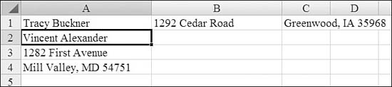
A co-worker has some names and addresses in Excel. She needs to do a mail merge in Word. Rather than teach her how to do a mail merge, you offer to do the mail merge for her. In theory, this should take you a couple minutes. However, when the list of names arrives in the Excel worksheet, you realize that the data is in the wrong format. In the Excel worksheet, the names are going down Column A, as shown in Figure 36.1.

Figure 36.1. A simple task such as doing a mail merge is incredibly difficult when the data is in the wrong format.

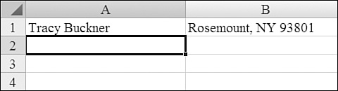
In order to successfully do a mail merge, the Excel worksheet should have fields for name, street address, and city+state+zip code, as shown in Figure 36.2.

Figure 36.2. The goal is to produce data with fields in columns.

Before you start recording a macro, you need to think about how to break the task into easily repeatable steps. The macro recorder is great at recording navigation done using arrow keys. Therefore, ideally, you want to use only the keyboard for navigation while using the macro recorder.

It would be good to record a macro that can fix one name in the list. Assume that you start with the cell pointer on a person’s name at the beginning of the macro, as shown in Figure 36.3. The macro would need to perform these steps to fix one record and end up on the name of the second person in the list:

Figure 36.3. You start with a name selected.

1. Press the Down Arrow key to move to the address cell.
2. Press Ctrl+X to cut the address.
3. Press the Up Arrow key and then the Right Arrow key to move next to the name.
4. Press Ctrl+V to paste the address, as shown in Figure 36.4.

   Figure 36.4. You cut and paste the address.

   

5. Press the Left Arrow key once and the Down Arrow key twice to move to the cell for city, state, and zip code.
6. Press Ctrl+X to cut the city, as shown in Figure 36.5.

   Figure 36.5. You cut the city.

   

7. Press the Up Arrow key twice and the Right Arrow key twice to move to the right of the street cell.
8. Press Ctrl+V to paste the city.
9. Press the Left Arrow key twice and the Down Arrow key once to move to the now blank row just below the name.
10. Hold down the Shift key while pressing the Down Arrow key twice in order to select the three blank rows, as shown in Figure 36.6.

    Figure 36.6. You select three blank rows prior to deleting.

    

11. Press Ctrl+- to invoke the delete command. Press R+Enter to delete the row.

When you run a macro that goes through these steps, Excel deletes the three blank rows, but the selection now contains the three cells that encompass the next record, as shown in Figure 36.7. Ideally, the macro should end with only the name selected. Therefore, the macro now needs to press the Up Arrow key and the Down Arrow key. Moving the cell pointer up a cell and then back to the name causes only a single cell to be selected, as shown in Figure 36.8.

Figure 36.7. You need only one cell selected instead of three.

Figure 36.8. You finish the macro with the cell pointer on the next name.

If the macro correctly performs all these steps, the first name and address are properly formatted. The blank rows left between the first and second names are deleted.

By making sure that the macro starts on a name and ends up on the next name, you allow the macro to be run repeatedly. If you assign this macro to the keyboard shortcut Ctrl+J, you can then hold down Ctrl+J and quickly fix records, one after the other.

How Not to Record a Macro: The Default State of the Macro Recorder

The default state of the macro recorder is a very stupid state. If you recorded the preceding steps in the macro recorder, the macro recorder would take your actions very literally. The English pseudocode for recording these steps would say this:

1. Move to Cell A2.
2. Cut Cell A2 and paste to Cell B1.
3. Move to Cell A3.
4. Cut Cell A3 and paste to Cell C1.
5. Delete Rows 2 through 4.
6. Select Cell A2.

This macro will work, but it will only work for one record. After you recorded this macro, your worksheet would look like the one shown in Figure 36.9.

Figure 36.9. After recording the macro in default mode, the first record is fixed, and you might think you are ready to run the macro to fix the second record.

When the default macro runs, it moves the name Vincent Alexander from Cell A2 and pastes it on top of the address in Cell B1. It then takes the address in Cell A3 and pastes it on top of the city in Cell C1. It then deletes Rows 2, 3, and 4, removing the city and state. As shown in Figure 36.10, the macro provides the wrong result.

Figure 36.10. When the default macro runs, it ruins two records.

If you blindly ran this macro 100 times to convert 100 addresses, the macro would happily “eat” all 100 records, leaving you with just one record (and not even a correct record), as shown in Figure 36.11.

Figure 36.11. Run the default macro 100 times, and it destroys your entire dataset. Luckily, there is a different mode available for recording relative macros, as described in the next section.

To overcome this problem, use relative references as discussed in the next section.

Relative References in Macro Recording

There is an icon in the Code group on the Developer tab on the ribbon called Use Relative References. The key to recording useful macros is to judiciously turn on and off the relative recording setting. If you performed the steps described in the preceding section in relative recording mode, Excel would write code that does this:

1. Move down one cell.
2. Cut that cell.
3. Move up and over one cell and paste.
4. Move left and down two cells.
5. Cut that cell.
6. Move up and over two cells and paste.
7. Move left two cells, move down one cell, and delete three rows.
8. Move up and down one cell in order to select a single cell.

These steps are far more generic than those recorded using the default state of the macro recorder and would work for any record, provided that you started the macro with the cell pointer on the first cell that contains a name.

For this example, you need to record the entire macro with relative recording turned on.

Starting the Macro Recorder

At this point, you have rehearsed the steps needed for a macro that puts data records into a format that will be usable for a mail merge. After you make sure that the cell pointer is starting on the name in Cell A1, you are ready to turn on the macro recorder.

You shouldn’t be nervous, but you really want to perform the steps correctly. If you move the cell pointer in the wrong direction, the macro recorder will happily record that for you and play it back. It would be annoying to watch the macro recorder play back your mistakes 100 times a day for the next five years, so follow these steps to correctly create the macro:

1. On the Developer tab of the ribbon, click the Record Macro icon from the Code group. The Record Macro dialog appears.
2. Excel suggests giving this macro the unimaginative name Macro1. You can use any name you want, up to 20 characters, and without spaces. For this example, name the macro FixOneRecord.
3. Choose a shortcut key for the macro. The shortcut key is very important. In the present example, you will have to run this macro once for each record, so you might choose something like Ctrl+A, which is easy to press. However, note that assigning a macro to Ctrl+A will overwrite the usual action of that keystroke (selecting all cells). If you are writing a macro that will be used all day every day, you should use a shortcut key that is not assigned to any existing shortcuts, such as Ctrl+J or Ctrl+K.
4. Make a selection from the Store Macro In drop-down. You have the option of storing the macro in this workbook, in a new workbook, or in the personal macro workbook. If this is a general-purpose macro that you will use everyday on every file, it would make sense to store the macro in the personal macro workbook. However, because this macro is going to be used just to solve a current problem, store it in the current workbook.
5. Fill in a description if you think you will be using this macro long enough to forget what it does. When you are done making selections on the Record Macro dialog (see Figure 36.12), click OK. The Record Macro icon changes to a Stop Recording icon.

   Figure 36.12. After making the needed selections, click OK to begin recording.

   

6. Click the Use Relative References icon in the Developer ribbon. The icon becomes highlighted.
7. Press the Down Arrow key to move to the address cell.
8. Press Ctrl+X to cut the address.
9. Press the Up Arrow key and then the Right Arrow key to move next to the name.
10. Press Ctrl+V to paste the address.
11. Press the Left Arrow key once and the Down Arrow key twice to move to the cell for city, state, and zip code.
12. Press Ctrl+X to cut the city
13. Press the Up Arrow key twice and the Right Arrow key twice to move to the right of the street cell.
14. Press Ctrl+V to paste the city.
15. Press the Left Arrow key twice and the Down Arrow key once to move to the now blank row just below the name.
16. Hold down the Shift key while pressing the Down Arrow key twice in order to select the three blank rows.
17. Press Ctrl+- to invoke the delete command. Press R+Enter to delete the row.
18. Press the Up Arrow key and the Down Arrow key. Moving the cell pointer up a cell and then back to the name will cause only a single cell to be selected.
19. When you are done, click the Stop Recording button.

This macro will successfully fix any record in the database, provided the cellpointer is on the cell containing the name when you run the macro. Try playing back the macro by pressing Ctrl+A to fix one record. To fix all records, hold down Ctrl+A until all records are fixed.

Running a Macro

To run a macro, you follow these steps:

1. Click the green triangle on the Code group of the Developer tab. The Macro dialog appears, as shown in Figure 36.13.

   Figure 36.13. Playing back a macro by using the Macro dialog.

   

2. Select your macro and click the Run button. The macro fixes the first record.

   Caution

   When you run a macro, there is no undo. Therefore, you should save a file before running a new macro on it. It is easy to have accidentally recorded the macro in default mode instead of relative mode. You need to save the macro so that you can easily go back to the current state in case something doesn’t work right.

3. Press Ctrl+A to run the FixOneRecord macro. As shown in Figure 36.14, the second record is fixed.

   Figure 36.14. Results of a successful macro.

   

4. Hold down Ctrl+A to repeatedly run the macro. In a matter of seconds, all 100 names are in a format that is ready to use in a mail merge.

This first example represents an ideal use of a one-time macro. Someone gave you data that was in a bad format. The process to fix the data involved mindless repetition. If there had just been four records, you could have easily mindlessly fixed the records. But because there were 100 records in this example, it made sense to quickly record a macro and then run the macro repeatedly to solve the problem. You recorded the entire macro in relative mode, and you did not have to edit the macro at all. You probably run into a few situations a week where a quick one-time-use macro would make your job easier.

Everyday-Use Macro Example: Formatting an Invoice Register

The macro recorder does not solve all tasks perfectly, however. Many times, you need to record a macro and then edit the recorded code to make the macro a bit more general. This example demonstrates how to do that.

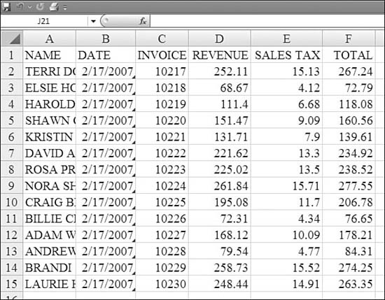
In this example, a system writes out a file every day. This file contains a list of invoices generated on the previous day. The file predictably contains six columns—NAME, DATE, INVOICE, REVENUE, SALES TAX, and TOTAL—as shown in Figure 36.15. The file also looks horrible: The columns are the wrong width, there is no title, there is not a total row at the bottom. You would like a macro that would open this file, make the columns wider, add a total row, add a title, make the headings bold, and save the file with a new name. The following sections describe how to create this macro.

Figure 36.15. You can create a macro to format this file every day.

Using the End Key to Handle a Variable Number of Rows

One of the inherent problems with this example is that your file will have a different number of rows every day. If you record a macro for this today to add totals in Row 16, it will not work tomorrow, when you might have 22 invoices. The solution is to use the End key to navigate to the last row of your data.

You use the End key to move to the edge of a contiguous range of data. In Figure 36.15, if you press the End key and then the Down Arrow key, you would move to Cell A15. If you press the End key and then the Up Arrow key, you move back to Cell A1. You can press the End key followed by the Right Arrow key to move to Cell F1.

You can also use the End key to jump over an abyss of empty cells. If you are currently at the edge of a range—for example, Cell F1—and press End followed by the Right Arrow key, Excel jumps over all the blank cells and stops either at the next nonblank cell in Row 1 or at the right edge of the worksheet, Cell XFD1.

You might be tempted to start in Cell A1, press End, press the Down Arrow key, and then press the Down Arrow key again to move to the first blank row in the data. However, that is the wrong thing to do. This data file is coming from another system. One day, I guarantee that some crazy cashier will find a way to enter an order without a customer name. She will happen upon the accidental keystroke combination that causes the cash register to allow an order without a customer name. On that day, the End+Down Arrow key combination will stop at the wrong row and add totals in the middle of your dataset. To prevent this problem, you should have the macro go through these steps:

1. Open the file.
2. Turn on absolute recording.
3. Press the F5 key to display the GoTo dialog.
4. Go to Cell A1048576 (the last cell in the worksheet).
5. Turn on relative recording.
6. Type End+Up Arrow to move to the last row that contains data.
7. Type the Down Arrow key to move to the blank row.
8. Type the word Total.
9. Move right three cells.
10. Hold down the Shift key while moving right two cells.
11. Click the AutoSum button.
12. Select all cells.
13. Choose Format, Column, AutoFit.
14. Turn on absolute recording.
15. Select Row 1.
16. Press Ctrl+B to apply bold.
17. Insert two rows.
18. Move to Cell A1.
19. Enter the formula ="Invoices for "&TEXT(B4,"mmmm d, yyyy").
20. Use Save As to save the file with a new name to reflect today’s date.
21. Click the Stop Recording button.

Before recording this macro, you need to open a blank Excel workbook and save it with the name MacroToImportInvoices.xlsm.

In this macro example, you use a mix of relative and absolute recording to produce a macro that handles any number of rows of data. The macro will be fairly useful, with two annoying limitations:

• If you saved the file as 2006-Feb-17Invoices.xls, the macro will attempt to overwrite that file everyday.
• The macro will always want to open the same file. This is great if your cash register system always produces a file with the same name in the same folder. However, you might want the option to browse for a different file each day.

Both of these changes require you to edit the recorded macro, as described in the next section.

Editing a Macro

To edit a macro, follow these steps:

1. Go to the Developer tab, and in the Code group, click the Macros button. The Macro dialog appears.
2. In the Macro dialog, select your macro and click Edit (see Figure 36.16). The Visual Basic Editor (VBE) is launched.

Figure 36.16. Launching the VBE through the Macro dialog is an easy way to make sure you find the proper code.

A number of panes are available in the VBE, but it is common to have three particular panes displayed, as shown in Figure 36.17:

• Code pane—The actual lines of the macro code are in the Code pane, which is usually on the right side of the screen.
• Project pane—This pane, in the upper left, shows every open workbook. Within the workbooks you can see objects for each worksheet, an object for this workbook, and one or more code modules. If you cannot see the Project pane, you press use Ctrl+R or select View, Project Explorer to open it.
• Properties pane—This pane, in the lower left, is very useful if you are designing custom dialog boxes. You can Press F4 to display the Properties pane.

Figure 36.17. The VBE allows editing of recorded macro code.

Understanding VBA Code—An Analogy

In the 1980s and early 1990s, many people going through school were exposed to an introductory class in a programming language called BASIC. Although Excel macros are written in Visual Basic for Applications, the fact that both languages contain the word basic does not mean that BASIC and VBA are the same or even similar. BASIC is a procedural language. VBA is an object-oriented language. In VBA, the focus is on objects. This can make VBA confusing to someone who has learned to program in BASIC.

The syntax of VBA is made up of objects, methods, collections, arguments, and properties. If you have never programmed in an object-oriented language, these terms, and the VBA code itself, might seem foreign to you. The following sections compare these five elements to parts of speech:

• An object is similar to a noun
• A method is similar to a verb
• A collection is similar to a plural noun
• An argument is similar to an adverb
• A property is similar to an adjective

Each of the following sections describe the similarity between the VBA element and a part of speech. It also describes how to recognize the various elements when you examine VBA Code.

Comparing Object.Method to Nouns and Verbs

As an object-oriented language, the objects in VBA are of primary importance. Think of an object as any noun in Excel. Examples of objects are a cell, a row, a column, a worksheet, and a workbook.

A method is any action that you can peform on an object. This is similar to a verb. You can add a worksheet. You can delete a row. You can clear a cell. In Excel VBA, words like “Add,” “Delete,” and “Clear,” are methods.

Objects and methods are joined together by a period, although in VBA, people pronounce the period as a dot. The object is first, followed by a dot, followed by the method. For example, object.method is pronounced “object-dot-method” and indicates that the method performs on the object. This is confusing because it is backward from how English is spoken. If we all spoke VBA instead of English, our day would be filled with sentences like “car.drive” and “dinner.eat.” When you see a period in VBA, it usually means that the word after the period is acting upon the word to the left of the period.

Comparing Collections to Plural Nouns

In an Excel workbook, there is not a single cell but a collection of many cells. Many workbooks will contain several worksheets. Anytime you have multiple instances of a certain object, VBA refers to this as a collection.

The “s” at the end of an object may seem subtle, but it indicates you are dealing with a collection instead of a single object. While This Workbook refers to a single workbook, Workbooks refers to a collection of all of the open workbooks. This is a very important distinction to understand.

There are two main ways to refer to a single worksheet in a collection of worksheets: You can refer to a worksheet by its number or by its name. For example, Worksheets(1) and Worksheets(“Jan”) might refer to the same worksheet.

Comparing Parameters to Adverbs

When you invoke a command such as the Save As command, a dialog box pops up, and you have the opportunity to specify several options that change how the command will be carried out. If the Save As command is a method, then the options for it are parameters. Just like an adverb modifies a verb, a parameter modifies a method.

Most of the time, parameters are recorded by using the syntax ParameterName:=ParameterValue.

One of the reasons that recorded code gets to be so long is that the macro recorder makes note of every option on the dialog box, whether you select it or not.

Consider this line of code for SaveAs:

In this recorded macro for SaveAs, the recorder noted parameter values for Filename, FileFormat, and CreateBackup. Figure 36.18 shows the Save As dialog box. Filename and FileFormat are clearly evident on the form, but where are the rest of those options?

Figure 36.18. It seems like the macro recorder is making up options that are not on the dialog box.

In the bottom corner of the dialog is a Tools drop-down. If you choose Tools and then General Options, you see a dialog box with four additional options, as shown in Figure 36.19. Even though you did not touch this Save Options dialog, Excel recorded the values in it for you.

Figure 36.19. Even though you did not touch the Save Options dialog box, the macro recorder recorded the values from it.

Parameters have some potentially confusing aspects. Most of the time, there is a space following the method and then a list of one or more ParameterName:=ParameterValue constructs, separated by a comma and a space. However, there are a couple exceptions:

• If the result of the method is acted upon by another method, the list of parameters is enclosed in parentheses, and there is no space after the method name. This commonly happens when you add a chart to a worksheet and then Excel selects the chart.
• When you use the parameter name, you can specify the parameters in any sequence you like. The Help topic for the method reveals the official default order for the parameters. If you specify the parameters in the exact sequence specified in Help, you are allowed to leave off the parameter names. However, this is a poor coding practice. Even if you’ve memorized the default order for the parameters, you can not assume that everyone else reading your code will know the default order. The problem is that sometimes the macro recorder will record code in this style. For example, here is a line of code that was recorded when I added WordArt to a worksheet:

  

  It would be very difficult to figure out this line of code without looking at the help topic. To access Help, you can click anywhere in the method of AddTextEffect. The help topic reveals that the correct parameter order is the one shown in Figure 36.20.

Figure 36.20. The Help topic for each method helps decode the default order of the parameters.

Again, parameters are like adverbs. They generally appear with a ParameterName:=ParameterValue construct, but there are times when the macro recorder lists the parameter values in their default order, without the parameter names or the :=.

Comparing Adjectives

The final construct in VBA is the adjective used to describe an object. In VBA, adjectives are called properties. Think about a cell in Excel with a formula in it. The cell has many properties. These are some of the most popular properties:

• Value (the value shown in the cell)
• Formula (the formula used to calculate Value)
• Font Name
• Font Size
• Font Color
• Cell Interior Color

In VBA, you can either check on the value of a property or you can set the property to a new value. To change several cells to be bold, for example, you would change their Bold property to true:

Selection.Font.Bold = True

You could also check to see if a property equals a certain value.

If Selection.Value = 100 then Selection.Font.Bold = True

Properties are generally used with the dot construct, and they are almost always followed by = (as contrasted with the := used with parameters). For example, PropertyName = value.

Using the Analogy While Examining Recorded Code

When you understand that a period generally separates an object from a method, you can start to make sense of the recorded code.

For example, the following line performs the Open method:

Workbooks.Open Filename:="C:Invoices.xls"

In this example, the Filename parameter is shown with := after the parameter name.

This first line in the following example performs the Select method on one particular member of the Rows collection:

The second line then sets the Bold property of the Font property of the selection to true. Using these two lines of code is equivalent to selecting Row 1 and clicking the Bold icon.

Using Simple Variables and Object Variables

The macro recorder never records a variable, but you can add variables to a macro when you edit the code. Let’s say that you need to do a number of operations to the row where the totals will be located. Rather than repeatedly going to the last row in the spreadsheet and pressing the End+Up Arrow, you could assign the row number to a variable:

The words FinalRow and TotalRow are variables that each hold a single value. If you have data in Rows 2 through 25 today, FinalRow will hold the value 25, and TotalRow will hold the value of 26. This allows you to use efficient code such as the following:

VBA also offers a powerful variable called an object variable. An object variable can be used to represent any object, such as a worksheet, a chart, or a cell. Whereas a simple variable holds one value, an object variable holds values for every property associated with the object.

Object variables are declared using the Dim statement and then assigned using the Set statement:

Using object variables offers several advantages. First, it is easier to refer to WSD than to ActiveWorkbook.Worksheets("Sheet1"). Second, if you define the object variable with a DIM statement at the beginning of the macro, as you type new lines of code, the VBE’s AutoComplete feature shows a list of valid methods and properties for the object, as shown in Figure 36.21.

Figure 36.21. Object variables hold many properties instead of a single value.

Using R1C1-Style Formulas

If you are a history buff, you might know that VisiCalc was the first spreadsheet program for PCs. When Dan Bricklin and Bob Frankston invented VisiCalc, they used the A1 style for naming cells. In those early days, VisiCalc had competitors such as SuperCalc and a Microsoft program called MultiPlan. This early Microsoft spreadsheet used the notation of R1C1 to refer to Cell A1. The cell that we know today as E17 would have been called R17C5, for Row 17, Column 5.

In 1985, Microsoft launched Excel version 1.0 for the Macintosh. Excel originally continued to use the R1C1 style of notation. During the next 10 years, Excel and Lotus 1-2-3 were locked in a bitter battle for market share. Lotus was the early leader, and it had adopted the A1 notation style familiar to VisiCalc customers. To capture more market share, Microsoft allowed Excel to use either A1-style notation or R1C1-style notation. Even today, in Excel 2007, you can turn on R1C1 style notation (by choosing Office Icon, Excel Options, Formulas, R1C1 Reference Style). Hardly anyone actually uses R1C1 reference style; however, the macro recorder always records formulas in R1C1 style.

Figure 36.22 shows the familiar formula =SUM(D$2:D15). When entered in Cell D16, this formula adds up everything from Row 2 to the row just above the current cell.

Figure 36.22. This familiar formula is in A1-style notation.

If you now turn on R1C1 style in this worksheet, the formula changes to =SUM(R2C:R[-1]C), as shown in Figure 36.23.

Figure 36.23. The formula in R1C1 notation would be confusing to most spreadsheet users.

In R1C1 notation, the reference RC refers to the current cell. You can modify RC by adding a particular row number or column number. For example, R2C refers to the cell in Row 2 of the current column. RC1 refers to the cell in this row that is in Column 1.

If you put a row number or column number in square brackets, it refers to a relative number of cells from the current cell. If you have a formula in Cell D16 and use the reference R[1]C[-2], you are referring to the cell one row below D16 and two columns to the left of D16, which would be cell B17.

You are probably wondering why the macro recorder uses this arcane notation style when recording formulas. It turns out that this style is fantastic for formulas. For example, take a look at the formulas in Column F of the worksheet, as shown in Figure 36.24. Every formula is a little different. When you copy F2 to F3, Excel has to change the references of E2 and D2 to be E3 and D3.

Figure 36.24. In A1 style, every formula in F2:F15 is different.

Now, look at these same formulas in R1C1 style, as shown in Figure 36.25. Every formula in that range is exactly identical. This makes sense: The formula is actually saying, “Add the sales tax one cell to the left of me to the merchandise amount that is two cells to the left of me.”

Figure 36.25. In R1C1 style, every formula in F2:F15 is identical.

If you were forced to use A1-style formulas in a macro, you might have to enter the formula in Cell F2 and then copy the formula from F2 to the remaining cells:

Instead, using R1C1 style formulas, you can enter all the formulas in one line of code:

Range("F2:F15").FormulaR1C1 = "=RC[-2]+RC[-1]"

If you are not yet convinced to learn how to use R1C1-style formulas, the final straw is that you have to use R1C1-style formulas when setting up conditional formatting in VBA.

Fixing Calculation Errors in Macros

Probably the most important reason to understand R1C1 formulas is to make sure that the macro recorder recorded the proper formula. Remember that when you recorded the macro described in the section “Using the End Key to Handle a Variable Number of Rows” earlier in this chapter, you had selected cells D16:F16 and clicked the AutoSum button. Excel recorded the following line of code:

Selection.FormulaR1C1 = "=SUM(R[-14]C:R[-1]C)"

This formula adds up a range from 14 rows above the selection to the cell just above the selection. This works only on days on which you have exactly 14 rows of data. This is one of the most annoying bugs in a macro. Although many times, a macro will return an error if you try to do something wrong, if you run this macro on tomorrow’s invoice file and there are 20 invoices, the macro will happily total only the last 14 invoices instead of all 20 invoices. You could easily distribute this report with a wrong total for several days before someone realizes that something is amiss.

It is easy to correct the formula. You know that you have headings in Row 1 and the first invoice will appear in Row 2. You need the macro to sum from Row 2 to the row just above the current cell. Therefore, you need to change the formula to this:

Selection.FormulaR1C1 = "=SUM(R2C:R[-1]C)"

Customizing the Everyday-Use Macro Example: GetOpenFileName and GetSaveAsFileName

The everyday-use macro you recorded earlier in this chapter (for formatting an invoice register) is hard-coded to always open the same file and to always save with the same filename. To make the macro more general, you might like to allow the person running the macro to browse for the file each morning and then to specify a new filename during the Save As. Excel offers a very easy way to display the File Open or File Save As dialog. Here is the code you need to use:

Note that this code displays the File Open dialog and allows a file to be selected. When you click Open, the dialog assigns the filename to the variable. It does not actually open the file. You then need to open the file specified in the variable:

Workbooks.Open Filename:=FileToOpen

When you want to ask for the filename to use in saving the file, use this code:

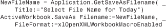
The following macro is the final macro to use each day:

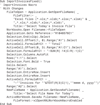
Out of the 19 lines in the macro, you needed to correct 1 line—the total formula. In order to add functionality, you added two lines and changed two other lines. This is fairly typical: Perhaps 10% to 20% of a recorded macro generally needs to be adjusted.

From-Scratch Macro Example: Loops, Flow Control, and Referring to Ranges

Say you work for a company that sells printers and scanners to commercial accounts. When you sell a piece of hardware, you also try to sell a service plan for that hardware. Customers in your state are taxed. Your accounting software provides a daily download that looks like Columns A:D in Figure 36.26.

Figure 36.26. Your accounting software groups all hardware, service, and tax amounts into a single column.

You want to create a macro that examines each row in the dataset and carries out a different action, based on the value in Column D. This is a macro that you will probably want to write from scratch. The following sections describe how you do it.

Looping Through All Rows

The loop most commonly used in VBA is a For-Next loop. This is identical to the loop that you might have learned about in a BASIC class.

In this example, the loop starts with a For statement. You specify that on each pass through the loop, a certain variable will change from a low value to a high value. This simple macro will run through the loop 10 times. On the first pass through the loop, the variable x will be equal to 1. The two lines inside the loop will assign the value 1 to Cells A1 and B1. When the macro encounters the Next x line, it will return to the start of the loop, increment x by 1, and run through the loop again. The next time through the loop, the value of x will be 2. Cell A2 will be assigned the number 2, and cell B2 will show 4 (which is the square of 2). Eventually, x will be equal to 10. At the Next x line, the macro will allow the loop to finish. The following is the code for this macro:

After you run this macro, you have a simple table that shows the numbers 1 through 10 and their squares, as shown in Figure 36.27

Figure 36.27. This simple loop fills in 10 rows.

After a loop is written, it is easy to adjust it. If you want a table showing all the squares from 1 to 100, you would simply adjust the For x = 1 to 10 line to be For x = 1 to 100.

There is an optional clause in the For statement called the step value. If no step value is shown, the program moves through the loop by incrementing the variable by 1 each time through the loop. If you wanted to check only the even-numbered rows, you could change the loop to be For x = 2 to 100 Step 2.

If you are going to be optionally deleting rows from a range of data, it is important to start at the bottom and proceed to the top of the range. You would use -1 as the step value:

For x = 100 to 1 step -1

Referring to Ranges

The macro recorder uses the Range property to refer to a particular range. You might see the macro recorder refer to ranges such as Range("B3") or Range("W1:Z100").

The loop code shown in the preceding section emulates this style of referring to ranges. On the third time through the loop, this line of code would refer to Cell B3:

Range("B" & x).value = x * x

But what if you wanted to loop through each column? How would you handle that? If you wanted to continue using the Range property, you would have to jump through some hoops to figure out the letter that is associated with Column 5:

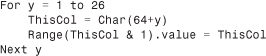
This method works fine if you are using only 26 or fewer columns. But if you needed to loop through all the columns out to Column XFD, you would spend all day trying to write the logic to assign the column label WMJ to Column 15896.

Instead of using the Range property, you can use the Cells property. Cells requires that you specify a numeric row number and a numeric column number. For example, Cell B3 would be specified as follows:

Cells(3, 2)

If you need to refer to a rectangular range, you can use the Resize property. Resize requires you to specify the number of rows and the number of columns. To refer to W1:Z100, for example, you would use this:

Cells(1, 23).Resize(100, 3)

It is certainly difficult to figure out that this refers to W1:Z100, but it allows you to easily loop through rows or columns.

You could use the following code to make every other column bold:

Combining a Loop with FinalRow

Earlier in this chapter, you learned how to use the End key to find the final row in a dataset. After finding the final row in the dataset and assigning it to a variable, you can specify that the loop should run through FinalRow:

Making Decisions by Using Flow Control

Flow control is the ability to make decisions within a macro. As described in the following sections, two commonly used flow control constructs are If-End If and Select Case.

Using the If-End If Construct

Say that you need a macro to delete any records that say Sales Tax. You could accomplish this with a simple If-End If construct:

This construct always starts with the word If, followed by a logical test, followed by the word Then. Every line between the first line and the End If line is executed only if the logical test is true.

Now say that you want to enhance the macro so that any other amounts that contain service plan revenue are moved to Column F. To do this, you use the ElseIf line to enter a second condition and block of lines to be used in that condition:

You could continue adding ElseIf statements to handle other situations. Eventually, just before the End If, you could add an Else block to handle any other condition that you haven’t thought about.

Using the Select Case Construct

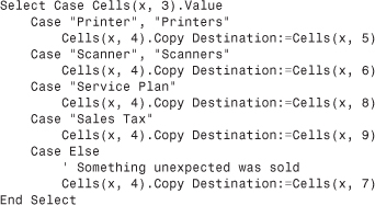
If you reach a point where you have many ElseIf statements all testing the same value, it might make sense to switch to a Select Case construct. To illustrate, say that you want to loop through all the records, examining the product in Column C. If Column C contains a printer, you want to move the amount in Column D to a new Column E. Scanner revenue should go to a new Column F. Service plans go to a new Column H. Sales tax goes to a new Column I. You should also handle the situation where something is sold and contains none of those products. In that case, you would move the revenue to a new Column G.

The construct begins with Select Case and then the value to check. The construct ends with End Select, which is similar to End If.

Each subblock of code starts with the word Case and one or more possible values. If you needed to check for Printer or Printers, you would enclose each in quotes and separate them with a comma.

After checking for all the possible values you can think of, you might add a Case Else subblock to handle any other stray values that might be entered in Column C.

The following code checks to see what product is in column C. Depending on the product, the program copies the revenue from column D to a specific column.

Putting Together the From-Scratch Example: Testing Each Record in a Loop

Using the building blocks described in the preceding sections, you can now write the code for a macro that finds the last row, loops through the records, and copies the total revenue to the appropriate column. Now you need to add new headings for the additional columns, as shown in Figure 36.28.

Figure 36.28. Adding new headings before running the macro.

The macro should use the End property to locate the final row. It should also prefill Columns E through I with 0s. Next, it should loop from Row 2 down to the final row. For each record, the revenue column should be moved to one of the columns. At the end of the loop, the program alerts you that the program is complete, using a MsgBox command. The following is the complete code of this macro:

After you run this macro, you see that the revenue amounts have been copied to the appropriate columns, as shown in Figure 36.29.

Figure 36.29. After running the macro, you have a breakout of revenue by product.

A Special Case: Deleting Some Records

If a loop will be conditionally deleting records, you will run into trouble if it is a typical For-Next loop. Let’s say you want to delete all the sales tax records, as follows:

Consider the data in Figure 36.30.

Figure 36.30. A forward-running loop encounters problems.

The first time through the loop, x is equal to 2. Cell C2 does not contain tax, so Cell E2 has the word checked. A similar result occurs for Rows 3 and 4. The fourth time through the loop, Cell C5 contains tax. The macro deletes the tax in Row 5. However, Excel then moves the old Row 6 up to Row 5, as shown in Figure 36.31. The next time through the loop, the program inspects Row 6, and the data that is now in Row 5 will never be checked.

Figure 36.31. The old Row 6 data moves up to occupy the deleted Row 5. This row will never be checked.

The macro succeeds in deleting tax, but several rows were never checked, and several extra blank rows at the bottom were needlessly checked, as shown in Figure 36.32.

Figure 36.32. Several rows went unchecked in this loop.

The solution is to have the loop run backward. You need to start at the final row and proceed up through the sheet to Row 2. When the macro deletes tax in Row 31, it can then proceed to checking Row 30, knowing that nothing has been destroyed (yet) in Row 30 and above.

To reverse the flow of the loop, you have to tell the loop to start at the final row, but you also have to tell the loop to use a step value of -1. The start of the loop would use this line of code:

For x = FinalRow to 2 Step -1

The macro needed here represents a fairly common task: looping through all the records in order to conditionally do something to each record.

The following macro correctly deletes all the sales tax records:

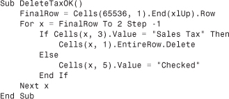
For the example described here, the macro recorder would be almost no help. You would have to write this simple macro from scratch. However, it is a powerful macro that can simplify tasks when you have hundreds of thousands of rows of data.

Combination Macro Example: Creating a Report for Each Customer

Many real-life scenarios require you to use a combination of recorded code and code written from scratch. For example, Figure 36.33 shows a dataset with all your invoices for the year. In this case, say you would like to produce a workbook for each customer that you can mail to the customer.

Figure 36.33. The goal is to provide a subset of this data to each customer.

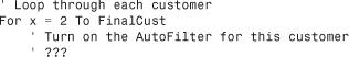
One way to handle this task would be to use an advanced filter to get a list of all unique customers in Column A. You would then loop through these customers, applying an AutoFilter to the dataset in order to see only the customers that match the selected customer. After the dataset is filtered, you could select the visible cells only and copy them to a new workbook. Then you could save the workbook with the name of the customer and then return to the original workbook.

You could start by creating a blank procedure with comments to spell out the steps in the preceding paragraphs. Then you would add in code for the loop and other simple tasks, such as copying the selection to a new workbook. Whenever you encounter a step that you’ve never written code for, you could just leave a comment with question marks. This would allow you to go back and record parts of the process in order to finish the macro.

Your first pass at a well-commented macro might look like this:

As described in the following sections, to create this macro, you need to figure out how to code the advanced filter to copy a unique list of customers to Column H. You then need to figure out how to apply a filter to Column A. Finally, you need to figure out how to select only the visible cells from the filter.

Using the Advanced Filter for Unique Records

You need to figure out how to use an advanced filter to finish the following section of code:

To use an advanced filter on this section of code, follow these steps:

1. Turn on the macro recorder.
2. On the Data tab, in the Sort & Filter group, click the Advanced icon to open the Advanced Filter dialog.
3. Choose the option Copy to Another Location.
4. Adjust the list range to refer only to Column A. The copy-to range will be Cell H1.
5. Check the Unique Records Only box.
6. When the dialog looks as shown in Figure 36.34, click OK. The result is a new range of data in Column H, with each customer listed just once, as shown in Figure 36.35.

   Figure 36.34. Using an advanced filter to get a unique list of customers.

   

   Figure 36.35. The advanced filter produces a list of customers for the macro to loop through.

   

7. On the Developer tab, click Stop Recording.
8. Use the Macros button to choose Macro1 and then select Edit.

Even though the Advanced Filter dialog is still one of the most complicated facets of Excel 2007, the recorded macro is remarkably simple:

In your macro, there is no reason to select Cell H1, so you can delete that line of code. The remaining problem is that the macro recorder hard-coded that today’s dataset contains 1,000 rows. You might want to generalize this to handle any number of rows. The follow code reflects these changes:

Using AutoFilter

When you have a list of customers, the macro will loop through each customer. The goal is to use an AutoFilter to display only the records for each particular customer. You now need to finish this section of code:

To apply an AutoFilter to this section of code, follow these steps:

1. On the Developer tab, choose Record Macro.
2. On the Home tab, choose the icon Sort & Filter – Filter. Drop-down arrows are turned on for each field.
3. In the drop-down in Cell A1, uncheck Select All and then check Hip Lawn Corporation.
4. Back on the Developer tab, stop recording the macro.
5. Use the Macros button to locate and edit Macro2 as follows:

   

The macro recorder always does too much selecting. You rarely have to select something before you can operate on it. You can theorize that the only line of this macro that matters is the Selection.AutoFilter line. Because you will always be looking at the AutoFilter drop-down in Cell A1, you can replace Selection with Range("A1"). Rather than continually ask for one specific customer, you can replace the end of the line with a reference to a cell in Column H:

Range("A1").AutoFilter Field:=1, Criteria1:=Cells(x, 8).Value

Selecting Visible Cells Only

After you use the AutoFilter in the macro, you see only records for one customer. However, as you can see in Figure 36.36, the other records are still there; they are just hidden. If you copied the range to a new worksheet, all the hidden rows would come along, and you would end up with 20 copies of your entire dataset.

Figure 36.36. If you copy this range to a new worksheet, the hidden rows copy as well.

The long way to select visible cells only is to press F5 to display the GoTo dialog. In the GoTo dialog, you click the Special button and then click Visible Cells Only. The shortcut, however, is to simply press Alt+;.

In order to learn how to select visible cells only in VBA, record the macro by following these steps:

1. Select the data in Columns A through F.
2. Turn on the macro recorder and press Alt+;.
3. Stop the macro recorder. You should see that the recorded macro has just one line of code:

   

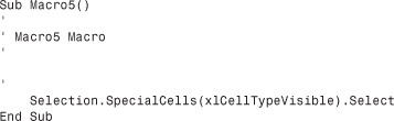
   In your original outline of the macro, you had contemplated selecting visible cells only and then doing the copy in another statement, like this:

   

   Instead, simply copy the visible cells in one statement:

   

The Combination Macro Example: Putting It All Together

The following macro started as a bunch of comments and a skeleton of a loop:

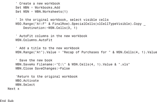
After doing three small tests with the macro recorder, you were able to fill in the sections to actually copy the customer records to a new workbook. After running this macro, you should have a new workbook for each customer on your hard drive, ready to be distributed via email.

Conclusion

VBA macros open up a wide possibility of automation for Excel worksheets. Any time that you are faced with a daunting, mindless task, you can turn it into a challenging exercise by trying to design a macro to do the task instead. It usually takes less time to design a macro than it does to complete the task. You should save every macro you write. Soon you will have a library of macros that handle many common tasks, and they will allow you to develop macros faster. The next time you need to perform a similar task, you can roll out the macro and perform the steps in seconds instead of hours.